Model fitting in R

Overview

Teaching: 15 min
Exercises: 5 min

Questions

• How do I fit a linear model in R?

• How do these fit in with the tidyverse way of working?

Objectives

• To understand how to fit a linear regression in R

• To understand how to integrate this into a tidyverse analysis pipeline

So far we’ve looked at exploratory analysis; loading our data, manipulating it and plotting it. We often wish to fit a statistical model to the data. The model(s) you need to fit will depend on your data and the questions you want to try and answer.

Fortunately, R will almost certainly include functions to fit the model you are interested in, either using functions in the stats package (which comes with R), a library which implements your model in R code, or a library which calls a more specialised modelling language. The CRAN task views are a good place to start if your preferred modelling approach isn’t included in base R.

In this episode we will very briefly discuss fitting linear models in R. The aim of this episode is to give a flavour of how to fit a statistical model in R, and to point you to further resources. The episode is based on modelling section of R for Data Science, by Grolemund and Wickham. For a more statistical and in-depth treatment, see, e.g. Linear Models with R, by Faraway.

As with the rest of the course, we’ll use the gapminder data. To make things a little more tractable, let’s consider only data for the UK:

gapminder_uk <- gapminder %>% 
  filter(country == "United Kingdom")

To start with, let’s plot GDP per capita as a function of time:

ggplot(data = gapminder_uk, aes(x=year, y=gdpPercap)) + geom_point()

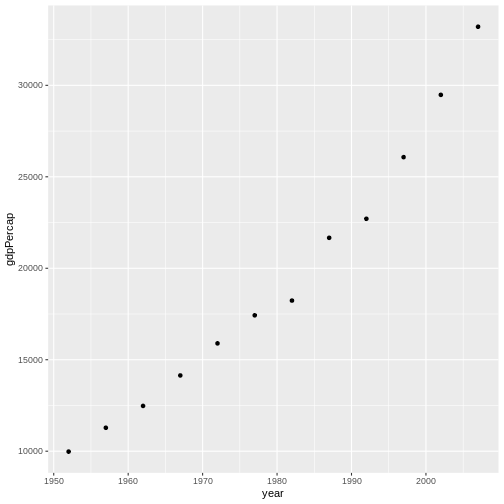
This looks like it’s (roughly) a straight line.

We can perform linear regression on the data using the lm() function:

lm(gdpPercap ~ year, data = gapminder_uk)

Call:
lm(formula = gdpPercap ~ year, data = gapminder_uk)

Coefficients:
(Intercept)         year  
  -777027.8        402.3  

This will fit the model:

We see that, according to the model, the UK’s GDP per capita is growing by $400 per year (the gapminder data has GDP in international dollars). The intercept gives us the model’s prediction of the GDP in year 0. This doesn’t make sense (the GDP has to be >0), and illustrates the perils of extrapolating from your data.

Saving your model

We can assign the model to a variable:

ukgdp_model <- lm(gdpPercap ~ year, data = gapminder_uk)
print(ukgdp_model)

Call:
lm(formula = gdpPercap ~ year, data = gapminder_uk)

Coefficients:
(Intercept)         year  
  -777027.8        402.3  

The summary() function will give us more details about the model.

summary(ukgdp_model)

Call:
lm(formula = gdpPercap ~ year, data = gapminder_uk)

Residuals:
    Min      1Q  Median      3Q     Max 
-2153.9  -786.3  -277.6   977.9  2758.8 

Coefficients:
              Estimate Std. Error t value Pr(>|t|)    
(Intercept) -777027.82   48840.08  -15.91 1.98e-08 ***
year            402.33      24.67   16.31 1.56e-08 ***
---
Signif. codes:  0 '***' 0.001 '**' 0.01 '*' 0.05 '.' 0.1 ' ' 1

Residual standard error: 1475 on 10 degrees of freedom
Multiple R-squared:  0.9638,	Adjusted R-squared:  0.9601 
F-statistic: 265.9 on 1 and 10 DF,  p-value: 1.563e-08

Fitting other terms

We can add additional terms to our model; ?formula() explains the syntax used. For example, to fit a covariate, z, giving the model

\[\mbox{gdpPercap} = x_0 + x_1 \times \mbox{year} + x_2 \times z\]

We would use:

ukgdp_model_squared <- lm(gdpPercap ~ year + z , data = gapminder_uk)

Note, however, if we wish to transform covariates you may need to use the I() function to prevent the transformation being interpreted as part of the model formula. For example, to fit:

\[\mbox{gdpPercap} = x_0 + x_1 \times \mbox{year} + x_2 \times \mbox{year}^2\]

We use:

ukgdp_model_squared <- lm(gdpPercap ~ year + I(year^2) , data = gapminder_uk)

This is because the ^ operator is used to fit models with interactions between covariates; see ?formula for full details.

Challenge 1: Modelling life expectancy

Using the gapminder_uk data, plot life-expectancy as a function of year. Assuming it is reasonable to fit a linear model to the data, do so. How much does the model suggest life expectancy increases per year?

Solution

We can plot life expectancy as a function of year as follows:

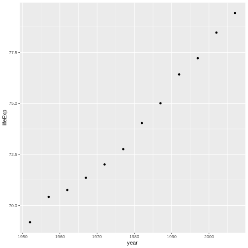
gapminder_uk %>% ggplot(aes(x=year, y=lifeExp)) + geom_point()

It looks like life expectancy has been increasing approximately linearly with time, so fitting a linear model is probably reasonable. We can do this with:

uk_lifeExp_model <- lm(lifeExp ~ year, data=gapminder_uk)

The summary() function will display information on the model:

summary(uk_lifeExp_model)

Call:
lm(formula = lifeExp ~ year, data = gapminder_uk)

Residuals:
     Min       1Q   Median       3Q      Max 
-0.69767 -0.31962  0.06642  0.36601  0.68165 

Coefficients:
              Estimate Std. Error t value Pr(>|t|)    
(Intercept) -2.942e+02  1.464e+01  -20.10 2.05e-09 ***
year         1.860e-01  7.394e-03   25.15 2.26e-10 ***
---
Signif. codes:  0 '***' 0.001 '**' 0.01 '*' 0.05 '.' 0.1 ' ' 1

Residual standard error: 0.4421 on 10 degrees of freedom
Multiple R-squared:  0.9844,	Adjusted R-squared:  0.9829 
F-statistic: 632.5 on 1 and 10 DF,  p-value: 2.262e-10

According to the model, life expectancy is increasing by 0.186 years per year.

Model predictions

Let’s compare the predictions of our model to the actual data. We can do this using the add_predictions() function in modelr. modelr is part of the tidyverse, but isn’t loaded by default.

library(modelr)

gapminder_uk %>% 
  add_predictions(ukgdp_model) %>% 
  ggplot(aes(x=year, y=pred)) + geom_line() +
  geom_point(aes(y=gdpPercap))

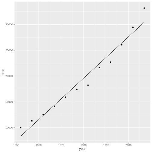
The model we have fitted assumes linear (i.e. straight line) change with respect to time. It looks like this is a not entirely unreasonable, although there are systematic differences. For example, the model predicts a larger GDP per capita than reality for all the data between 1967 and 1997.

Parameter uncertainty

Unfortunately add_predictions() doesn’t show the uncertainty in our model. If we wish to calculate confidence or prediction intervals we need to use the predict() function.

Model checking – plotting residuals

We can formalise this a little more by plotting the model residuals.

Briefly - residuals show us “what’s left over” after fitting the model. If the model fits well we would expect these to be randomly distributed (i.e. no systematic patterns).

Extensive details on model checking and diagnostics are beyond the scope of the episode - in practice we would want to do much more, and also consider and compare the goodness of fit of other models.

We can add the model residuals to our tibble using the add_residuals() function in modelr.

gapminder_uk %>% 
  add_residuals(ukgdp_model) %>% 
  ggplot(aes(x = year, y = resid)) + geom_point()

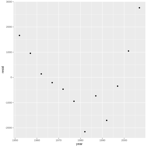
This makes the systematic difference between our model’s predictions and reality much more obvious. If the model fitted well we would expect the residuals to appear randomly distributed about 0.

Challenge 2:

Plot the residuals for your life expectancy model. Do they appear random?

Advanced: Try adding a quadratic term to your model? Does this appear to improve the model fit? (in practice we would want to compare the models more formally).

Having plotted the residuals, plot the model predictions and the data. If you made a model with a quadratic term, you might wish to compare the two models’ predictions. The var= option of add_predictions() will let you override the default variable name of pred.

Solution 2:

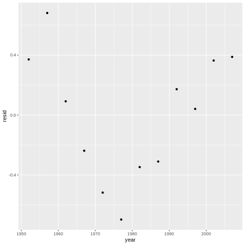
We can calculate model residuals using add_residuals(). By including this in a pipeline we can immediately plot them.

gapminder_uk  %>% 
  add_residuals(uk_lifeExp_model) %>% 
  ggplot(aes(x=year, y=resid)) + 
  geom_point()  

It looks like values towards the centre of our year range are under-estimated, while values at the edges of the range are over estimated. The plot of the data from challenge 1 suggests suggests that there is some curvature in the data.

We can fit a linear model with a year squared term as follows:

uk_lifeExp_model_squared <- lm(lifeExp ~ year + I(year^2), data=gapminder_uk)

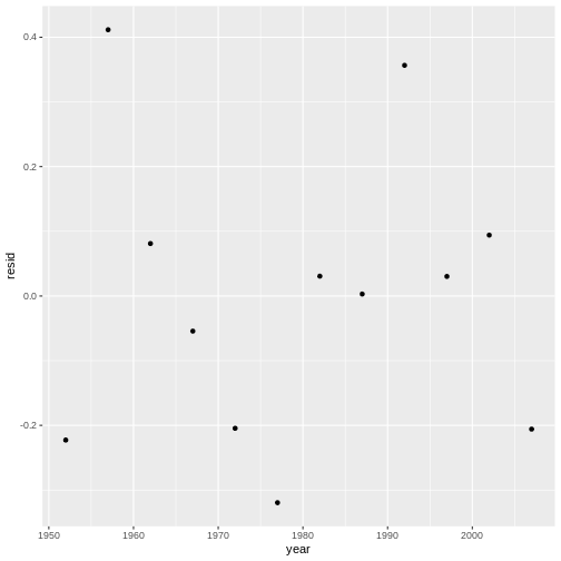
gapminder_uk %>% add_residuals(uk_lifeExp_model_squared) %>% 
  ggplot(aes(x=year, y=resid)) + 
  geom_point()  

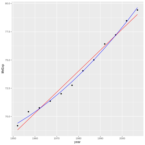
The distribution of the residuals appears much more random. We can visually compare the two models by generating predictions from them both, and plotting (note that we use the var option to override the default variable name for the predictions):

gapminder_uk %>% add_predictions(uk_lifeExp_model, var="linear") %>% 
  add_predictions(uk_lifeExp_model_squared, var="squared") %>% 
  ggplot(aes(x=year, y=lifeExp)) + geom_point() +
  geom_line(aes(y=linear), colour="red") +
  geom_line(aes(y=squared), colour="blue")

Going further

This episode has barely scratched the surface of model fitting in R. Fortunately most of the more complex models we can fit in R have a similar interface to lm(), so the process of fitting and checking is similar.

The book R for Data Science, which this section is based on, is a very useful resource, and is freely available. The content is regularly updated to reflect current good practice.

Quick R provides a good overview of various standard statistical models and more advanced statistical models.

If you wish to fit Bayesian models in R, RStan provides an interface to the Stan programming language. The rstanarm package provides an lm() like interface to many common statistical models implemented in Stan, letting you fit a Bayesian model without having to code it from scratch.

If you are interested in machine learning approaches, the keras package provides an R interface to the Keras library.

Key Points

• The lm() function fits a linear model

• summary() gives details of the fitted model

• We can use add_predictions() and add_residuals() to generate model predictions and calculate residuals