Visualisation

Last updated on 2023-09-11 | Edit this page

Overview

Questions

“How does an image with pleural effusion differ from one without?”
“How is image data represented in a NumPy array?”

Objectives

“Visually compare normal X-rays with those labelled with pleural effusion.”
“Understand how to use NumPy to store and manipulate image data.”
“Compare a slice of numerical data to its corresponding image.”

Key Points

“In NumPy, RGB images are usually stored as 3-dimensional arrays.”

Visualising the X-rays

In the previous section, we set up a dataset comprising 700 chest X-rays. Half of the X-rays are labelled “normal” and half are labelled as “pleural effusion”. Let’s take a look at some of the images.

PYTHON

# cv2 is openCV, a popular computer vision library
import cv2
from matplotlib import pyplot as plt 
import random

def plot_example(example, label, loc):
    image = cv2.imread(example)
    im = ax[loc].imshow(image)
    title = f"Class: {label}\n{example}"
    ax[loc].set_title(title)

fig, ax = plt.subplots(1, 2)
fig.set_size_inches(10, 10)

# Plot a "normal" record
plot_example(random.choice(normal_list), "Normal", 0)

# Plot a record labelled with effusion
plot_example(random.choice(effusion_list), "Effusion", 1)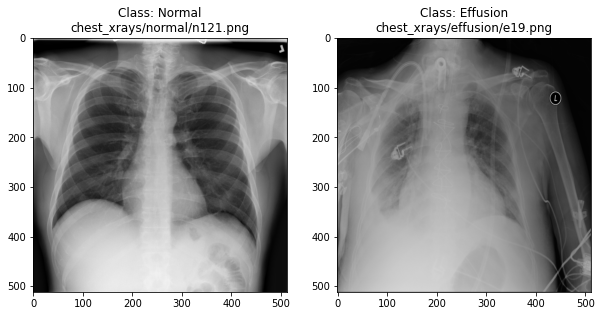

Can we detect effusion?

Run the following code to flip a coin to select an x-ray from our collection.

PYTHON

print("Effusion or not?")

# flip a coin
coin_flip = random.choice(["Effusion", "Normal"])
if coin_flip == "Normal":
    fn = random.choice(normal_list)
else:
    fn = random.choice(effusion_list)

# plot the image
image = cv2.imread(fn)
plt.imshow(image)

Show the answer:

PYTHON

# Jupyter doesn't allow us to print the image until the cell has run,
# so we'll print in a new cell.
print(f"The answer is: {coin_flip}!")

Exercise: Manual classification

Run the coin flip code 10 times and each time try to identify by eye whether the images are effusion or not. Make a note of your predictive accuracy >(hint: for a reminder of the formula for accuracy, check the solution below).

Show me the solution

Accuracy is the fraction of predictions that were correct (correct predictions / total predictions). > If you made 10 predictions and 5 were correct, your accuracy is 50%.

How does a computer see an image?

Consider an image as a matrix in which the value of each pixel corresponds to a number that determines a tone or color. Let’s load one of our images:

PYTHON

import numpy as np 

file_idx = 56
example = normal_list[file_idx]
image = cv2.imread(example)

print(image.shape)

OUTPUT

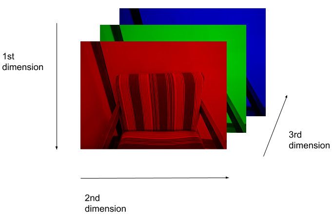
(512, 512, 3)

Here we see that the image has 3 dimensions. The first dimension is height (512 pixels) and the second is width (also 512 pixels). The presence of a third dimension indicates that we are looking at a color image (“RGB”, or Red, Green, Blue).

For more detail on image representation in Python, take a look at the Data Carpentry course on Image Processing with Python. The following image is reproduced from the section on Image Representation.

For simplicity, we’ll instead load the images in greyscale. A greyscale image has two dimensions: height and width. Each value in the matrix represents a tone between black (0) and white (255).

PYTHON

image = cv2.imread(example, cv2.IMREAD_GRAYSCALE)
print(image.shape)

OUTPUT

(512, 512)

Let’s briefly display the matrix of values, and then see how these same values are rendered as an image.

PYTHON

# Print a 10 by 10 chunk of the matrix
print(image[35:45, 30:40])

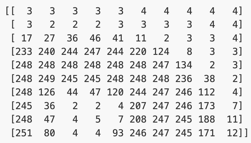
PYTHON

# Plot the same chunk as an image
plt.imshow(image[35:45, 30:40], cmap='gray', vmin=0, vmax=255)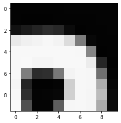

Image pre-processing

In the next episode, we’ll be building and training a model. Let’s prepare our data for the modelling phase. For convenience, we’ll begin by loading all of the images and corresponding labels and assigning them to a list.

PYTHON

# create a list of effusion images and labels
dataset_effusion = [cv2.imread(fn, cv2.IMREAD_GRAYSCALE) for fn in effusion_list]
label_effusion = np.ones(len(dataset_effusion))

# create a list of normal images and labels
dataset_normal = [cv2.imread(fn, cv2.IMREAD_GRAYSCALE) for fn in normal_list]
label_normal = np.zeros(len(dataset_normal))

# Combine the lists
dataset = dataset_effusion + dataset_normal
labels = np.concatenate([label_effusion, label_normal])

Let’s also downsample the images, reducing the size from (512, 512) to (256,256).

PYTHON

# Downsample the images from (512,512) to (256,256)
dataset = [cv2.resize(img, (256,256)) for img in dataset]

# Check the size of the reshaped images
print(dataset[0].shape)

# Normalize the data
# Subtract the mean, divide by the standard deviation.
for i in range(len(dataset)):
  dataset[i] = (dataset[i] - np.average(dataset[i], axis= (0, 1))) / np.std(dataset[i], axis= (0, 1))

OUTPUT

(256, 256)

Finally, we’ll convert our dataset from a list to an array. We are expecting it to be (700, 256, 256). That is 700 images (350 effusion cases and 350 normal), each with a dimension of 256 by 256.

PYTHON

dataset = np.asarray(dataset, dtype=np.float32)
print(f"Matrix Dimensions: {dataset.shape}")

OUTPUT

(700, 256, 256)

We could plot the images by indexing them on dataset, e.g., we can plot the first image in the dataset with:

PYTHON

idx = 0
vals = dataset[idx].flatten()
plt.imshow(dataset[idx], cmap='gray', vmin=min(vals), vmax=max(vals))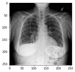

MATLAB

Initializing an Array

We just talked about how matlab thinks in arrays, and declared some very simple arrays using square brackets. In some cases, we will want to create space to save data, but not save anything just yet. One way of doing so is with zeros. The function zeros takes the dimensions of our array as arguments, and populates it with zeros. For example,

MATLAB

>> Z = zeros(3,5)

OUTPUT

Z =
     0     0     0     0     0
     0     0     0     0     0
     0     0     0     0     0

creates a matrix of 3 rows and 5 columns, all with zeros. If we had only passed one dimension, matlab assumes you want a square matrix, so

MATLAB

>> Z = zeros(3)

OUTPUT

Z =
     0     0     0
     0     0     0
     0     0     0

yields a 3x3 array. If we want a single row and 5 columns, we need to remember that matlab reads rowsxcolumns, so

MATLAB

>> Z = zeros(1x5)

OUTPUT

Z =
     0     0     0     0     0

This logic of the zeros function is shared with many other functions that create arrays.

For example, the ones function is quite similar, but the arrays are filled with ones, and the rand function assigns uniformly distributed random numbers between zero and 1.

MATLAB

>> R = rand(8);
>> O = ones(10,10);

Callout

Note: This is when supressing the output becomes more important. You can more comfortably explore the variables R and O by double clicking them in the workspace.

By the way, the ones function can actually help us initialize a matrix to any value, because we can multiply a matrix by a constant and it will multiply each element. So for example,

MATLAB

>> Fives = ones(3,6)*5;

Produces a 3x6 matrix full of fives.

The magic function has a similar logic, but you can only declare square matrices with it. The magic thing about them is that the sum of the elements on each row or column add up to the same number.

MATLAB

>> M = magic(4)

OUTPUT

M =
    16     2     3    13
     5    11    10     8
     9     7     6    12
     4    14    15     1

In this case, each row or column add up to 34. But how could I tell in a bigger matrix? How can I select some of the elements of the array and sum them, for example?

Array indexing

Array indexing, is the method by which we can select one or more different elements of an array. A solid understanding of array indexing will be essential to work with arrays. Lets start with selecting one element.

First, we will create an 8x8 “magic” matrix:

MATLAB

>> M = magic(8)

OUTPUT

ans =

   64    2    3   61   60    6    7   57
    9   55   54   12   13   51   50   16
   17   47   46   20   21   43   42   24
   40   26   27   37   36   30   31   33
   32   34   35   29   28   38   39   25
   41   23   22   44   45   19   18   48
   49   15   14   52   53   11   10   56
    8   58   59    5    4   62   63    1

We want to access a single value from the matrix:

To do that, we must provide its index in parentheses. In a 2D array, this means the row and column of the element separated by a comma, that is, as (row, column). This index goes after the name of our array. In our case, this is:

MATLAB

>> M(5, 6)

OUTPUT

ans = 38

So the index (5, 6) selects the element on the fifth row and sixth column of M.

Callout

Note: Matlab starts counting indices at 1, not 0! (as many other programming languages).

An index like the one we used selects a single element of an array, but we can also select a group of them if instead of a number we give arrays as indices. For example, if we want to select this submatrix:

we want rows 4, 5 and 6, and columns 5, 6 and 7, that is, the arrays [4,5,6] for rows, and [5,6,7] for columns:

MATLAB

>> M([4,5,6],[5,6,7])

OUTPUT

ans =
   36   30   31
   28   38   39
   45   19   18

The `:` operator

In matlab, the symbol : (colon) is used to specify a range. The range is specified as start:end. For example, if we type 1:6 it generates an array of consecutive numbers from 1 to 6:

MATLAB

>> 1:6

OUTPUT

ans =
   1     2     3     4     5     6

We can also specify an increment other than one. To specify the increment, we write the range as start:increment:end. For example, if we type 1:3:15 it generates an array starting with 1, then 1+3, then 1+2*3, and so on, until it reaches 15 (or as close as it can get to 15 without going past it):

MATLAB

>> 1:3:15

OUTPUT

ans =
   1     4     7    10    13

The array stopped at 13 because 13+3=16, which is over 15.

The rows and columns we just selected could have been specified as ranges. So if we want the rows from 4 to 6 and columns from 5 to 7, we can specify the ranges as 4:6 and 5:7. On top of being a much quicker and neater way to get the rows and columns, matlab knows that the range will produce an array, so we do not even need the square brackets anymore. So the command above becomes:

MATLAB

>> M(4:6, 5:7)

OUTPUT

ans =
   36   30   31
   28   38   39
   45   19   18

Checkerboard

Select the elements highlighted on the image:

Show me the solution

We need to select every other element in both dimensions. To do that, we define the apropriate intervals with an increment of 2:

MATLAB

>> M(1:3:8, 2:2:8)

OUTPUT

ans =
    2   61    6   57
   26   37   30   33
   15   52   11   56

Selecting whole rows or columns

If we want a whole row, for example:

we could in principle pick the 5th row and for the columns use the range 1:8.

MATLAB

>> M(5, 1:8)

OUTPUT

ans =
   32   34   35   29   28   38   39   25

However, we need to know that there are 8 columns, which is not very robust.

The key-word `end`

When indexing the elements of an array, the key word end can be used to get the last index available.

For example, M(2,end) returns the last element of the second row:

MATLAB

>> M(2,end)

OUTPUT

ans =
   16

We can also use it in combination with the : operator. For example, M(5:end,3) returns the elements of column 3 from row 5 until the end:

MATLAB

>> M(5:end,3)

OUTPUT

We can then use the keyword end instead of the 8 to get the whole row with 1:end.

MATLAB

>> M(5, 1:end)

OUTPUT

ans =
   32   34   35   29   28   38   39   25

This is much better, now this works for any size of matrix, and we don’t need to know the size.

Using `:` as an index

getting a whole row or column is such a common operation, that matlab has a shortcut: Using : alone is equivalent!

For example, We can then get the whole fifth row with:

MATLAB

>> M(5, :)

OUTPUT

ans =
   16

As you can see, the : operator is quite important when accessing arrays!

We can use it to select multiple rows,

MATLAB

>> M(1:4, :)

OUTPUT

ans =
   64    2    3   61   60    6    7   57
    9   55   54   12   13   51   50   16
   17   47   46   20   21   43   42   24
   40   26   27   37   36   30   31   33

or multiple columns:

MATLAB

>> M(:, 6:end)

OUTPUT

ans =
    6    7   57
   51   50   16
   43   42   24
   30   31   33
   38   39   25
   19   18   48
   11   10   56
   62   63    1

Master indexing

Select the elements highlighted on the image without using the numbers 5 or 8, and using end only once:

Show me the solution

We need to tart with row 2, and subsequently select every third row:

MATLAB

>> M(2:3:end, :)

OUTPUT

ans =
    9   55   54   12   13   51   50   16
   32   34   35   29   28   38   39   25
    8   58   59    5    4   62   63    1

Slicing character arrays

A subsection of an array is called a slice. We can take slices of character arrays as well:

MATLAB

>> element = 'oxygen';
>> disp(['first three characters: ', element(1:3)])
>> disp(['last three characters: ', element(4:6)])

OUTPUT

first three characters: oxy
last three characters: gen

Use slicing to:

Select all elements from the 3rd to the last one.
Find out what is the value of element(1:2:end)?
Figure out how would you get all characters except the first and last?

We used the single colon operator : in the indices to get all the available column or row numbers, but we can also use it like this: M(:). What do you think will happen? How many elements does M(:) have? What would happen if we use it for the element variable? Compare the result from element and element(:). Are there any differences?

Show me the solution

Exercises using slicing

To select all elements from 3rd to last we can use start our range at 3 and use the keyword end: matlab >> element(3:end) output ans = 'ygen'
The command element(1:2:end) starts at the first character, selects every other element (notice the interval is 2), and goes all the way until the last element, so: matlab >> element(1:2:end) output ans = 'oye'
To select each character starting with the second we set the start at 2, and to not include the last one we can finish at end-1: matlab >> element(2:end-1) output ans = 'xyge'

The colon operator gets all the elements that it can find, and so using it as M(:) returns all the elements of M. We can make sure that the result of M(:) has 8x8=64 elements by using the function size, which returns the dimensions of the array given as an input:
MATLAB
```
>> size(M(:))
```
OUTPUT
```
ans =
    64    1
```
So it has 64 rows and 1 column. Efectively, then, M(:) ‘flattens’ the array into a column vector. The order of the elements in the resulting vector comes from appending each column of the original array in turn. Therefore, the last 8 elements we see if we evaluate M(:) correspond to the last column of M, for example.

The difference between evaluating element and element(:) is that the former is a row vector, and the latter a column vector.

Key Points

“Some functions to initialize matrices include zeros, ones, and rand. They all produce a square matrix if only one argument is given, but you can specify the dimensions you want separated by a comma.”
“To select data points we use M(rows, columns), where rows and columns are the indices of the elements we want. They can be just numbers or arrays of numbers.”
“We use the colon operator to select ranges of elements as start:end or start:increment:end.”
“We use the keyword end to get the index of the last element.”
“The colon operator by itself : selects all the elements.”

Visualisation

Overview

Questions

Objectives

Key Points

Visualising the X-rays

PYTHON

Can we detect effusion?

PYTHON

PYTHON

Exercise: Manual classification

Show me the solution

How does a computer see an image?

PYTHON

OUTPUT

PYTHON

OUTPUT

PYTHON

PYTHON

Image pre-processing

PYTHON

PYTHON

OUTPUT

PYTHON

OUTPUT

PYTHON

MATLAB

Initializing an Array

MATLAB

OUTPUT

MATLAB

OUTPUT

MATLAB

OUTPUT

MATLAB

Callout

MATLAB

MATLAB

OUTPUT

Array indexing

MATLAB

OUTPUT

MATLAB

OUTPUT

Callout

MATLAB

OUTPUT

The : operator

MATLAB

OUTPUT

MATLAB

OUTPUT

MATLAB

OUTPUT

Checkerboard

Show me the solution

MATLAB

OUTPUT

Selecting whole rows or columns

MATLAB

OUTPUT

The key-word end

MATLAB

OUTPUT

MATLAB

OUTPUT

MATLAB

OUTPUT

Using : as an index

MATLAB

OUTPUT

MATLAB

OUTPUT

MATLAB

OUTPUT

Master indexing

Show me the solution

MATLAB

OUTPUT

Slicing character arrays

The `:` operator

The key-word `end`

Using `:` as an index