Content from Introduction
Last updated on 2023-09-07 | Edit this page
Overview
Questions
- “What kinds of diseases can be observed in chest X-rays?”
- “What is pleural effusion?”
Objectives
- “Gain awareness of the NIH ChestX-ray dataset.”
- “Load a subset of labelled chest X-rays.”
Key Points
- “Algorithms can be used to detect disease in chest X-rays.”
Chest X-rays
Chest X-rays are frequently used in healthcare to view the heart, lungs, and bones of patients. On an X-ray, broadly speaking, bones appear white, soft tissue appears grey, and air appears black. The images can show details such as:
- Lung conditions, for example pneumonia, emphysema, or air in the space around the lung.
- Heart conditions, such as heart failure or heart valve problems.
- Bone conditions, such as rib or spine fractures
- Medical devices, such as pacemaker, defibrillators and catheters. X-rays are often taken to assess whether these devices are positioned correctly.
In recent years, organisations like the National Institutes of Health have released large collections of X-rays, labelled with common diseases. The goal is to stimulate the community to develop algorithms that might assist radiologists in making diagnoses, and to potentially discover other findings that may have been overlooked.
The following figure is from a study by Xiaosong Wang et al. It illustrates eight common diseases that the authors noted could be be detected and even spatially-located in front chest x-rays with the use of modern machine learning algorithms.
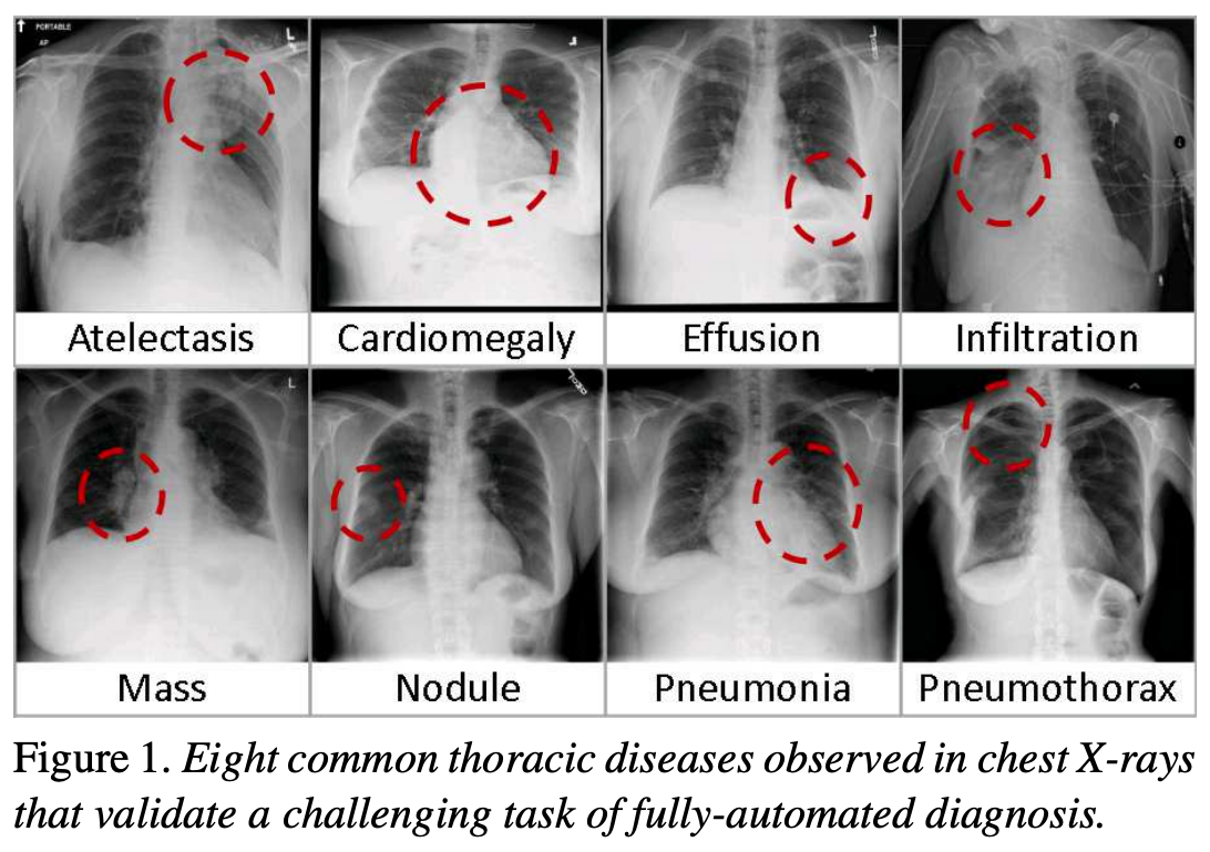
Pleural effusion
Thin membranes called “pleura” line the lungs and facilitate breathing. Normally there is a small amount of fluid present in the pleura, but certain conditions can cause excess build-up of fluid. This build-up is known as pleural effusion, sometimes referred to as “water on the lungs”.
Causes of pleural effusion vary widely, ranging from mild viral infections to serious conditions such as congestive heart failure and cancer. In an upright patient, fluid gathers in the lowest part of the chest, and this build up is visible to an expert.
For the remainder of this lesson, we will develop an algorithm to detect pleural effusion in chest X-rays. Specifically, using a set of chest X-rays labelled as either “normal” or “pleural effusion”, we will train a neural network to classify unseen chest X-rays into one of these classes.
Loading the dataset
The data that we are going to use for this project consists of 350 “normal” chest X-rays and 350 X-rays that are labelled as showing evidence pleural effusion. These X-rays are a subset of the public NIH ChestX-ray dataset.
Xiaosong Wang, Yifan Peng, Le Lu, Zhiyong Lu, Mohammadhadi Bagheri, Ronald Summers, ChestX-ray8: Hospital-scale Chest X-ray Database and Benchmarks on Weakly-Supervised Classification and Localization of Common Thorax Diseases, IEEE CVPR, pp. 3462-3471, 2017
Let’s begin by loading the dataset.
PYTHON
# The glob module finds all the pathnames matching a specified pattern
from glob import glob
import os

# If your dataset is compressed, unzip with:
# !unzip chest_xrays.zip

# Define folders containing images
data_path = os.path.join("chest_xrays")
effusion_path = os.path.join(data_path, "effusion", "*.png")
normal_path = os.path.join(data_path, "normal", "*.png")

# Create list of files
effusion_list = glob(effusion_path)
normal_list = glob(normal_path)

print('Number of cases with pleural effusion: ', len(effusion_list))
print('Number of normal cases: ', len(normal_list))
OUTPUT
Number of cases with pleural effusion:  350
Number of normal cases:  350
MATLAB
Introduction to the MATLAB GUI
Before we can start programming, we need to know a little about the MATLAB interface. Using the default setup, the MATLAB desktop contains several important sections:
- In the Command Window we can execute commands.
Commands are typed after the prompt
>>and are executed immediately after pressing Enter. - Alternatively, we can open the Editor, write our code and run it all at once. The advantage of this is that we can save our code and run it again in the same way at a later stage.
- The Workspace contains all the variables which we have loaded into memory.
- The Current Folder window shows files in the current directory, and we can change the current folder using this window.
-
Search Documentation on the top right of your
screen lets you search for functions. Suggestions for functions that
would do what you want to do will pop up. Clicking on them will open the
documentation. Another way to access the documentation is via the
helpcommand — we will return to this later.
Working with variables
In this lesson we will learn how to manipulate the inflammation dataset with MATLAB. But before we discuss how to deal with many data points, we will show how to store a single value on the computer.
We can create a new variable by
assigning a value to it using =:
OUTPUT
x =
    55
Notice that matlab responded by printing an output confirming that the variable has the desired value, and also that the variable appeared in the workspace.
A variable is just a name for a piece of data or value.
Variable names must begin with a letter, and are case sensitive. They
can contain also numbers or underscores. Examples of valid variable
names are weight, size3,
patient_name or alive_on_day_3.
The reason we work with variables is so that we can reuse them, or save them for later use. We can do operations with these variables. For example, we can do a simple sum:
OUTPUT
y =
    10
ans =
    65
Note that the answer was saved in a new variable called
ans. This variable is temporary, and will be overwritten
with any new operation we do. For example, if we now substract y from x
we get:
OUTPUT
ans =
    45
The result of the sum is now gone forever. We can of course assign the result of an operation to a new variable, for example:
OUTPUT
z =
    550
This created a new variable z. If you look at the
workspace, you can see that the value of z is 550.
We can even use a variable in an operation, and save the value in the same variable. Fer example:
OUTPUT
y =
    2
Where you can see that the expression to the right of the
= sign is evaluated first, and the result is then
assigned to the variable specified to the left of the =
sign.
Of course, we can use multiple variables in a single operation, for example:
OUTPUT
z =
    817
where we used the caret symbol ^ to take the third power
of y.
Logical operations
In programming, there is another type of opperation that becomes very important: comparison. We can compare two numbers (or variables) to see which one is smaller, for example
OUTPUT
c1 =
  logical
   1
Something interesting just happened with the variable c1. If I ask
you wether frac (8) is smaller than 10, you would say “yes”. Matlab
answered with a logical 1. If I ask you wether frac is
greater than 10, you would say “no”. Matlab answers with a
logical 0.
OUTPUT
c2 =
  logical
   0
There are only two options (yes or no, true or false, 0 or 1), and so it is “cheaper” for the computer to only save space for those two options.
The “type” of data is not the same as a number. It comes froma logical comparison, and so matlab identifies it as such.
You can also see that in the workspace these variables have a tick next to them, instead of the squares we had seen. There is actually other symbols we can get there, which relate to the types of information we can save (unfold the info below if you want to know more).
Data types
We mentioned above that we can get other symbols in the workspace which relate to the types of information we can save.
We know we can save numbers, and logical values, but we can also save letters or strings, for example. Numbers are by default saved as type double, which just means they can store very big or very small numbers. Letters are type ‘char’, and words or sentences are “strings”. Logical values (or booleans) are values that mean true or false, and are represented with zero or one. They are usually the result of comparing things.
OUTPUT
weight =
   64.5000
size3 =
    'L'
patient_name =
    "Jane Doe"
alive_on_day_3 =
  logical
   1
Notice the single tick for character variables, in contrast with the double quote for strings.
If you look at the woorkspace, you’ll notice that the icon next to each variable is different, and if you hover over it, it will tell you the type of variable it is.
We can also check if two variables (or even operations) are the same
OUTPUT
c3 =
  logical
   1
And we can combine comparisons. For example, we can check wether frac is smaller than 10 and the age is greater than 5
>> c4 = frac < 10 && age > 5
```matlab
```output
c4 =
  logical
   0
In this case, both conditions need to be met for the result to be “yes” (1).
If we want a “yes” as long as at least one of the conditions are met, we woudl ask if frac is smaller than 10 or the age is greater than 5
OUTPUT
c5 =
  logical
   1
Negating conditions and including the limits
We often asks questions or characterise things in negative. “We did not start late today.”, “I was not going faster than the speed limit officer!”, and “I didn’t shoot no deputy” are just some examples.
Naturally, we may want to do so in programming too. In matlab the
negative is represented with ~. For example, we can check
if the speed is indeed not faster than the limit with
~(speed > 70), which matlab reads as “not speed greater
than 70”.
Can you express these questions in matlab code? - Is 1 + 2 + 3 + 4 not smaller than 10? - Is 5 to the power of 3 different from 125? - Is x + y not greater or equal to x/y?
We can ask the first two question in positive, encapsulate it in
brackets, and then negate it: - ~(1 + 2 + 3 + 4 < 10) -
~(5^3 == 125)
Asking if two things are different is so common, that matlab has a
special symbol for it. So the second question, we could have asked
instead with - 5^3 ~= 125
- We can ask if x+y is greater or equal to x/y with
x+y > x/y || x+y == x/y, so asking if x + y not greater or equal to x/y we do by negating the above with brackets:~(x+y > x/y || x+y == x/y)
That last one seems a bit too complicated, and it is all beacuse we
need to include the limit, that is, because we want to include
values that are greater and equal to
something. There is actually a special symbol in matlab for that
>=, and of cours for smaller or equal too
<=.
Using this symbol, our last answer becomes
~(x+y >= x/y), which does not look nearly as scary.
Arrays
You may notice that all of the variable types start with a
1x1. This is because matlab thinks in terms of
groups of variables called arrays, or matrices.
We can create an array using square brackets and separating each value with a comma:
OUTPUT
A =
     1     2     3
If you now hover over the data type icon, you’ll find that it shows
1x3. This means that the array A has 1
row and 3
columns.
We can create matrices using semi-colons to separate rows:
OUTPUT
B =
     1     2
     3     4
     5     6
You’ll notice that B has three rows and two columns, which explains
the 3x2 we get from the workspace.
We can also create arrays of other types of data. For example, we could create an array of names:
OUTPUT
Names =
  1×4 string array
    "Jhon"    "Abigail"    "Bertrand"    "Lucile"
Or we can use logical values too:
OUTPUT
C =
  4×1 logical array
   1
   0
   0
   1
Something to bear in mind, however, is that all values in an array must be of the same type.
I mentioned before that matlab is actually used to working with arrays rather than individual variables. Well, if it is so used to them, can we do operations with them?
The answer is of course yes! In fact, this is what makes MATLAB a particularly interesting programming language.
We can, for example, check the whole matrix B and look for values greater than, say, 3.
OUTPUT
ans =
  3×2 logical array
   0   0
   0   1
   1   1
Matlab then compared each element of B and asked “is this element greater than 3?”. The result is another array, of the same size and dimensions as B, with the answers.
We can also do sums, multiplications, and pretty much anything we want with an array, but we need to be careful with what we do.
Despite this being so interesting and increadibly powerful, this course will focus on more basic programming concepts, and so we will use the feature rather little. However, it is very important that you keep it in mind, and that you do ask questions about it during the break if you are interested.
Suppressing the output
In general, the output can be a bit redundant (or even annoying!), and it can make the code slower, so it is considered good form to always supress it. To supress it, we add a semi-colon at the end of the line:
At first glance nothing appears to have happened, but the workspace shows the new value was assigned.
Printing a variable’s value
If we really want to print the variable, then we can simply type its name and hit Enter,
OUTPUT
patient_name =

    "Jane Doe"
or using the disp
function.
Functions are pre-defined algorithms (chunks of code), that can be used multiple times. They usually take some “inputs” inside brackets, and either produce something or output something.
The disp function, in particular, takes just one input – the variable that you want to print – and what it does is to print the variable in a nice way. For the variable patient_name, we would use it like this:
OUTPUT
Jane DoeNote how the output is a bit different from what we got when we just typed the variable name. There is less indentation and less empty lines.
Keeping things tidy
We have declared a few variables now, and we might not be using all
of them. If we want to delete a variable we can do so by typing
clear and the name of the variable, e.g.:
You might be able to see it disappear from the workspace. If you now try to use alive_on_day_3, matlab will error.
We can also delete all our variables with the
command clear, without any variable names. Be careful
though, there’s no way back!
Another thing you might want to clear every once in a while is the
output. To do that, we use the command clc.
Again, there is no way back!
Key Points
- “Variables store data for future use. Their names must start with a letter, and can have underscores and numbers.”
- “We can add, substract, multiply, divide and potentiate numbers.”
- “We can also compare variables with
<,>,==,>=,<=,~=, and use~to negate the result.” - “MATLAB stores data in arrays. The data in an array has to be of the same type.”
- “You can supress output with
;, and print a variable withdisp.” - “Use
clearto delete variables, andclcto clear the console.”
Content from Visualisation
Last updated on 2023-09-11 | Edit this page
Overview
Questions
- “How does an image with pleural effusion differ from one without?”
- “How is image data represented in a NumPy array?”
Objectives
- “Visually compare normal X-rays with those labelled with pleural effusion.”
- “Understand how to use NumPy to store and manipulate image data.”
- “Compare a slice of numerical data to its corresponding image.”
Key Points
- “In NumPy, RGB images are usually stored as 3-dimensional arrays.”
Visualising the X-rays
In the previous section, we set up a dataset comprising 700 chest X-rays. Half of the X-rays are labelled “normal” and half are labelled as “pleural effusion”. Let’s take a look at some of the images.
PYTHON
# cv2 is openCV, a popular computer vision library
import cv2
from matplotlib import pyplot as plt
import random

def plot_example(example, label, loc):
    image = cv2.imread(example)
    im = ax[loc].imshow(image)
    title = f"Class: {label}\n{example}"
    ax[loc].set_title(title)

fig, ax = plt.subplots(1, 2)
fig.set_size_inches(10, 10)

# Plot a "normal" record
plot_example(random.choice(normal_list), "Normal", 0)

# Plot a record labelled with effusion
plot_example(random.choice(effusion_list), "Effusion", 1)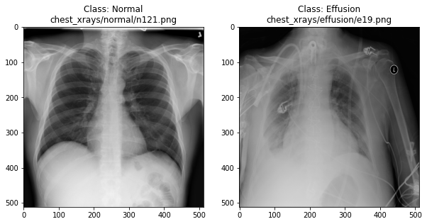
Can we detect effusion?
Run the following code to flip a coin to select an x-ray from our collection.
PYTHON
print("Effusion or not?")

# flip a coin
coin_flip = random.choice(["Effusion", "Normal"])
if coin_flip == "Normal":
    fn = random.choice(normal_list)
else:
    fn = random.choice(effusion_list)

# plot the image
image = cv2.imread(fn)
plt.imshow(image)
Show the answer:
PYTHON
# Jupyter doesn't allow us to print the image until the cell has run,
# so we'll print in a new cell.
print(f"The answer is: {coin_flip}!")
Exercise: Manual classification
- Run the coin flip code 10 times and each time try to identify by eye whether the images are effusion or not. Make a note of your predictive accuracy >(hint: for a reminder of the formula for accuracy, check the solution below).
- Accuracy is the fraction of predictions that were correct (correct predictions / total predictions). > If you made 10 predictions and 5 were correct, your accuracy is 50%.
How does a computer see an image?
Consider an image as a matrix in which the value of each pixel corresponds to a number that determines a tone or color. Let’s load one of our images:
PYTHON
import numpy as np

file_idx = 56
example = normal_list[file_idx]
image = cv2.imread(example)

print(image.shape)
OUTPUT
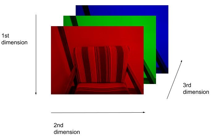
(512, 512, 3)Here we see that the image has 3 dimensions. The first dimension is height (512 pixels) and the second is width (also 512 pixels). The presence of a third dimension indicates that we are looking at a color image (“RGB”, or Red, Green, Blue).
For more detail on image representation in Python, take a look at the Data Carpentry course on Image Processing with Python. The following image is reproduced from the section on Image Representation.
For simplicity, we’ll instead load the images in greyscale. A greyscale image has two dimensions: height and width. Each value in the matrix represents a tone between black (0) and white (255).
OUTPUT
(512, 512)Let’s briefly display the matrix of values, and then see how these same values are rendered as an image.
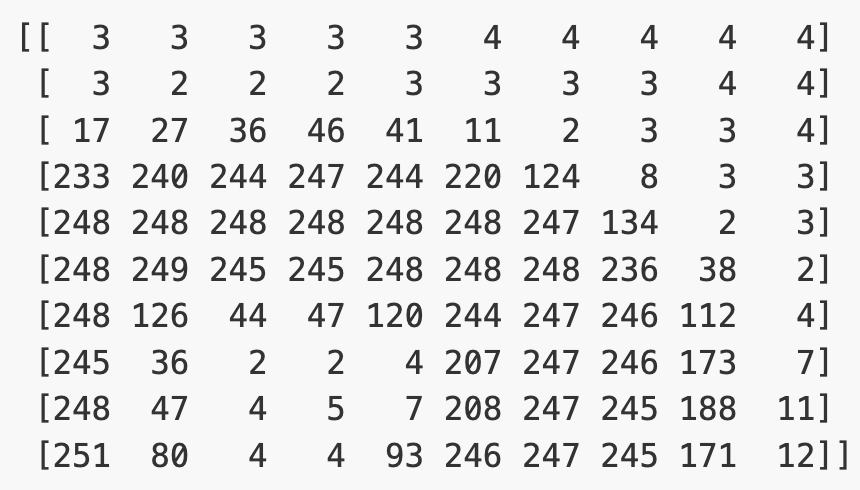
PYTHON
# Plot the same chunk as an image
plt.imshow(image[35:45, 30:40], cmap='gray', vmin=0, vmax=255)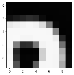
Image pre-processing
In the next episode, we’ll be building and training a model. Let’s prepare our data for the modelling phase. For convenience, we’ll begin by loading all of the images and corresponding labels and assigning them to a list.
PYTHON
# create a list of effusion images and labels
dataset_effusion = [cv2.imread(fn, cv2.IMREAD_GRAYSCALE) for fn in effusion_list]
label_effusion = np.ones(len(dataset_effusion))

# create a list of normal images and labels
dataset_normal = [cv2.imread(fn, cv2.IMREAD_GRAYSCALE) for fn in normal_list]
label_normal = np.zeros(len(dataset_normal))

# Combine the lists
dataset = dataset_effusion + dataset_normal
labels = np.concatenate([label_effusion, label_normal])
Let’s also downsample the images, reducing the size from (512, 512) to (256,256).
PYTHON
# Downsample the images from (512,512) to (256,256)
dataset = [cv2.resize(img, (256,256)) for img in dataset]

# Check the size of the reshaped images
print(dataset[0].shape)

# Normalize the data
# Subtract the mean, divide by the standard deviation.
for i in range(len(dataset)):
  dataset[i] = (dataset[i] - np.average(dataset[i], axis= (0, 1))) / np.std(dataset[i], axis= (0, 1))
OUTPUT
(256, 256)Finally, we’ll convert our dataset from a list to an array. We are expecting it to be (700, 256, 256). That is 700 images (350 effusion cases and 350 normal), each with a dimension of 256 by 256.
OUTPUT
(700, 256, 256)We could plot the images by indexing them on dataset,
e.g., we can plot the first image in the dataset with:
PYTHON
idx = 0
vals = dataset[idx].flatten()
plt.imshow(dataset[idx], cmap='gray', vmin=min(vals), vmax=max(vals))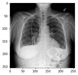
MATLAB
Initializing an Array
We just talked about how matlab thinks in arrays, and
declared some very simple arrays using square brackets. In some cases,
we will want to create space to save data, but not save anything just
yet. One way of doing so is with zeros. The function zeros
takes the dimensions of our array as arguments, and populates it with
zeros. For example,
OUTPUT
Z =
     0     0     0     0     0
     0     0     0     0     0
     0     0     0     0     0
creates a matrix of 3 rows and 5 columns, all with zeros. If we had only passed one dimension, matlab assumes you want a square matrix, so
OUTPUT
Z =
     0     0     0
     0     0     0
     0     0     0
yields a 3x3 array. If we want a single row and 5 columns, we need to
remember that matlab reads rowsxcolumns,
so
OUTPUT
Z =
     0     0     0     0     0
This logic of the zeros function is shared with many
other functions that create arrays.
For example, the ones
function is quite similar, but the arrays are filled with ones, and
the rand
function assigns uniformly distributed random numbers between zero
and 1.
Callout
Note: This is when supressing the output becomes
more important. You can more comfortably explore the variables
R and O by double clicking them in the
workspace.
By the way, the ones function can actually help us
initialize a matrix to any value, because we can multiply a matrix by a
constant and it will multiply each element. So for example,
Produces a 3x6 matrix full of fives.
The magic
function has a similar logic, but you can only declare square
matrices with it. The magic thing about them is that the sum of the
elements on each row or column add up to the same number.
OUTPUT
M =
    16     2     3    13
     5    11    10     8
     9     7     6    12
     4    14    15     1
In this case, each row or column add up to 34. But how could I tell in a bigger matrix? How can I select some of the elements of the array and sum them, for example?
Array indexing
Array indexing, is the method by which we can select one or more different elements of an array. A solid understanding of array indexing will be essential to work with arrays. Lets start with selecting one element.
First, we will create an 8x8 “magic” matrix:
OUTPUT
ans =

   64    2    3   61   60    6    7   57
    9   55   54   12   13   51   50   16
   17   47   46   20   21   43   42   24
   40   26   27   37   36   30   31   33
   32   34   35   29   28   38   39   25
   41   23   22   44   45   19   18   48
   49   15   14   52   53   11   10   56
    8   58   59    5    4   62   63    1
We want to access a single value from the matrix:

To do that, we must provide its index in
parentheses. In a 2D array, this means the row and column of the element
separated by a comma, that is, as (row, column). This index
goes after the name of our array. In our case, this is:
OUTPUT
ans = 38So the index (5, 6) selects the element on the fifth row
and sixth column of M.
Callout
Note: Matlab starts counting indices at 1, not 0! (as many other programming languages).
An index like the one we used selects a single element of an array, but we can also select a group of them if instead of a number we give arrays as indices. For example, if we want to select this submatrix:

we want rows 4, 5 and 6, and columns 5, 6 and 7, that is, the arrays
[4,5,6] for rows, and [5,6,7] for columns:
OUTPUT
ans =
   36   30   31
   28   38   39
   45   19   18
The : operator
In matlab, the symbol : (colon)
is used to specify a range. The range is specified as
start:end. For example, if we type 1:6 it
generates an array of consecutive numbers from 1 to 6:
OUTPUT
ans =
   1     2     3     4     5     6
We can also specify an increment other than one. To specify
the increment, we write the range as start:increment:end.
For example, if we type 1:3:15 it generates an array
starting with 1, then 1+3, then 1+2*3, and so on, until it reaches 15
(or as close as it can get to 15 without going past it):
OUTPUT
ans =
   1     4     7    10    13
The array stopped at 13 because 13+3=16, which is over 15.
The rows and columns we just selected could have been specified as
ranges. So if we want the rows from 4 to 6 and columns from 5 to 7, we
can specify the ranges as 4:6 and 5:7. On top
of being a much quicker and neater way to get the rows and columns,
matlab knows that the range will produce an array, so we do not even
need the square brackets anymore. So the command above becomes:
OUTPUT
ans =
   36   30   31
   28   38   39
   45   19   18
Checkerboard
Select the elements highlighted on the image:

Selecting whole rows or columns
If we want a whole row, for example:

we could in principle pick the 5th row and for the columns use the
range 1:8.
OUTPUT
ans =
   32   34   35   29   28   38   39   25
However, we need to know that there are 8 columns, which is not very robust.
The key-word end
When indexing the elements of an array, the key word end
can be used to get the last index available.
For example, M(2,end) returns the last element of the
second row:
OUTPUT
ans =
   16
We can also use it in combination with the : operator.
For example, M(5:end,3) returns the elements of column 3
from row 5 until the end:
OUTPUT
ans =
   35
   22
   14
   59
We can then use the keyword end instead of the 8 to get
the whole row with 1:end.
OUTPUT
ans =
   32   34   35   29   28   38   39   25
This is much better, now this works for any size of matrix, and we don’t need to know the size.
As you can see, the : operator is quite important when
accessing arrays!
We can use it to select multiple rows,

OUTPUT
ans =
   64    2    3   61   60    6    7   57
    9   55   54   12   13   51   50   16
   17   47   46   20   21   43   42   24
   40   26   27   37   36   30   31   33
or multiple columns:

OUTPUT
ans =
    6    7   57
   51   50   16
   43   42   24
   30   31   33
   38   39   25
   19   18   48
   11   10   56
   62   63    1
Master indexing
Select the elements highlighted on the image without using the
numbers 5 or 8, and using end only once:

Slicing character arrays
A subsection of an array is called a slice. We can take slices of character arrays as well:
MATLAB
>> element = 'oxygen';
>> disp(['first three characters: ', element(1:3)])
>> disp(['last three characters: ', element(4:6)])
OUTPUT
first three characters: oxy
last three characters: gen- Use slicing to:
- Select all elements from the 3rd to the last one.
- Find out what is the value of
element(1:2:end)? - Figure out how would you get all characters except the first and last?
- We used the single colon operator
:in the indices to get all the available column or row numbers, but we can also use it like this:M(:). What do you think will happen? How many elements doesM(:)have? What would happen if we use it for the element variable? Compare the result fromelementandelement(:). Are there any differences?
- Exercises using slicing
To select all elements from 3rd to last we can use start our range at
3and use the keywordend:matlab >> element(3:end)output ans = 'ygen'The command
element(1:2:end)starts at the first character, selects every other element (notice the interval is 2), and goes all the way until the last element, so:matlab >> element(1:2:end)output ans = 'oye'To select each character starting with the second we set the start at
2, and to not include the last one we can finish atend-1:matlab >> element(2:end-1)output ans = 'xyge'
-
The colon operator gets all the elements that it can find, and so using it as
M(:)returns all the elements of M. We can make sure that the result ofM(:)has 8x8=64 elements by using the function size, which returns the dimensions of the array given as an input:OUTPUT
ans =
    64    1
So it has 64 rows and 1 column. Efectively, then,
M(:)‘flattens’ the array into a column vector. The order of the elements in the resulting vector comes from appending each column of the original array in turn. Therefore, the last 8 elements we see if we evaluateM(:)correspond to the last column ofM, for example.The difference between evaluating
elementandelement(:)is that the former is a row vector, and the latter a column vector.
Key Points
- “Some functions to initialize matrices include zeros, ones, and rand. They all produce a square matrix if only one argument is given, but you can specify the dimensions you want separated by a comma.”
- “To select data points we use
M(rows, columns), where rows and columns are the indices of the elements we want. They can be just numbers or arrays of numbers.” - “We use the colon operator to select ranges of elements as
start:endorstart:increment:end.” - “We use the keyword
endto get the index of the last element.” - “The colon operator by itself
:selects all the elements.”
Content from Data preparation
Last updated on 2023-09-11 | Edit this page
Overview
Questions
- “What is the purpose of data augmentation?”
- “What types of transform can be applied in data augmentation?”
Objectives
- “Generate an augmented dataset”
- “Partition data into training and test sets.”
Partitioning into training and test sets
As we have done in previous projects, we will want to split our data into subsets for training and testing. The training set is used for building our model and our test set is used for evaluation.
To ensure reproducibility, we should set the random state of the splitting method. This means that Python’s random number generator will produce the same “random” split in future.
PYTHON
from sklearn.model_selection import train_test_split

# Our Tensorflow model requires the input to be:
# [batch, height, width, n_channels]
# So we need to add a dimension to the dataset and labels.
#
# Ellipsis (...) is shorthand for selecting with ":" across dimensions.
# np.newaxis expands the selection by one dimension.
dataset = dataset[..., np.newaxis]
labels = labels[..., np.newaxis]

# Create training and validation datasets in a 70:15:15 split
dataset_train, dataset_temp, labels_train, labels_temp = train_test_split(dataset, labels, test_size=0.3, stratify=labels, random_state=42)
dataset_val, dataset_test, labels_val, labels_test = train_test_split(dataset_temp, labels_temp, test_size=0.5, stratify=labels_temp, random_state=42)

print("No. images, x_dim, y_dim, colors) (No. labels, 1)\n")
print(f"Train: {dataset_train.shape}, {labels_train.shape}")
print(f"Validation: {dataset_val.shape}, {labels_val.shape}")
print(f"Test: {dataset_test.shape}, {labels_test.shape}")
OUTPUT
No. images, x_dim, y_dim, colors) (No. labels, 1)

Train: (505, 256, 256, 1), (505, 1)
Validation: (90, 256, 256, 1), (90, 1)
Test: (105, 256, 256, 1), (105, 1)
Data Augmentation
We have a small dataset, which increases the chance of overfitting our model. If our model is overfitted, it becomes less able to generalize to data outside the training data.
To artificially increase the size of our training set, we can use
ImageDataGenerator. This function generates new data by
applying random transformations to our source images while our model is
training.
PYTHON
from tensorflow.keras.preprocessing.image import ImageDataGenerator

# Define what kind of transformations we would like to apply
# such as rotation, crop, zoom, position shift, etc
datagen = ImageDataGenerator(
    rotation_range=0,
    width_shift_range=0,
    height_shift_range=0,
    zoom_range=0,
    horizontal_flip=False)
For the sake of interest, let’s take a look at some examples of the augmented images!
PYTHON
# specify path to source data
path = os.path.join("chest_xrays")
batch_size=5

val_generator = datagen.flow_from_directory(
        path, color_mode="rgb",
        target_size=(256, 256),
        batch_size=batch_size)

def plot_images(images_arr):
    fig, axes = plt.subplots(1, 5, figsize=(20,20))
    axes = axes.flatten()
    for img, ax in zip(images_arr, axes):
        ax.imshow(img.astype('uint8'))
    plt.tight_layout()
    plt.show()

augmented_images = [val_generator[0][0][0] for i in range(batch_size)]
plot_images(augmented_images)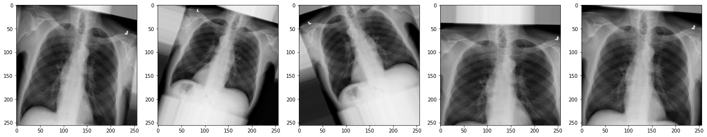
The images look a little strange, but that’s the idea! When our model sees something unusual in real-life, it will be better adapted to deal with it.
Now we have some data to work with, let’s start building our model.
MATLAB
Loading data to an array
Reading data from files and writing data to them are essential tasks in scientific computing, and something that we’d rather not spend a lot of time thinking about. Fortunately, MATLAB comes with a number of high-level tools to do these things efficiently, sparing us the grisly detail.
Before we get started, however, let’s create some directories to help organise this project.
Tip: Good Enough Practices for Scientific Computing
Good Enough Practices for Scientific Computing is a paper written by researchers involved with the Carpentries, which covers basic workflow skills for research computing. It recommends the following for project organization:
- Put each project in its own directory, which is named after the project.
- Put text documents associated with the project in the
docdirectory. - Put raw data and metadata in the
datadirectory, and files generated during clean-up and analysis in aresultsdirectory. - Put source code for the project in the
srcdirectory, and programs brought in from elsewhere or compiled locally in thebindirectory. - Name all files to reflect their content or function.
We already have a data directory in our
matlab-novice-inflammation project directory, so we only
need to create results and src directories for
this project. You can use your computer’s file browser to create this
directory.
A final step is to set the current folder in MATLAB to our project folder. Use the Current Folder window in the MATLAB GUI to browse to your project folder (the one now containing the ‘data’ and ‘results’ directories).
To verify the current directory in matlab we can run pwd
(print working directory). A second check we can do is to run the
ls (list) command in the Command Window to list the
contents of the working directory — we should get the following
output:
OUTPUT
data results srcWe are now set to load our data.
If we know what our data looks like (in this case, we have a matrix
stored as comma-separated values) and we’re unsure about what command we
want to use, we can search the documentation. Type
read matrix into the documentation toolbar. MATLAB suggests
using readmatrix. If we have a closer look at the
documentation, MATLAB also tells us, which inputs and output this
function has.
For the readmatrix function we need to provide a single
argument: the path to the file we want to read
data from. Since our data is in the ‘data’ folder, the path will begin
with “data/”, and will be followed by the name of the file:
This loads the data and assigns it to a variable, patient_data. This is a good example of when to use a semi-colon to suppress output — try re-running the command without the semi-colon to find out why. You should see a wall of numbers printed, which is the data from the file.
We can see in the workspace that the variable has 60 rows and 40
columns. If you can’t see the workspace, you can check this with
size, as we did before:
OUTPUT
ans =
    60 40
You might also recognise the icon in the workspace telling you that
the variable is of type double. If you don’t, you can use the
class function to find out what type of data lives inside
an array:
OUTPUT
ans =
    'double'
Again, this just means that you can store very small or very large numbers, called double precision floating-point numbers.
Initial exploration
We know that in our data each row represents a patient and each column a different day.
One patient at a time
We know how to access sections of our data, so lets look at a single patient first. If we want to look at a single patients’ data, then, we have to get all the columns for a given row, with:
OUTPUT
patient_5 =
  Columns 1 through 25
     0     1     1     3     3     1     3     5     2     4     4     7     6     5     3    10     8    10     6    17     9    14     9     7    13
  Columns 26 through 40
     9    12     6     7     7     9     6     3     2     2     4     2     0     1     1
Looking at these 40 numbers tells us very little, so we might want to look at the mean instead, for example.
OUTPUT
mean_p5 =
    5.5500
We can also compute other statistics, like the maximum, minimum and standard deviation.
OUTPUT
max_p5 =
    17
min_p5 =
     0
std_p5 =
    4.1072
All data points at once
Can you think of a way to get the mean of the whole data? What about
the max, min and std?
We already know that the colon operator as an index returns all the
elements, so patient_data(:) will return a vector with all
the data points. To compute the mean, we then use:
OUTPUT
global_mean =
    6.1487
This works for max, min and
std too:
MATLAB
>> global_max = max(patient_data(:))
>> global_min = min(patient_data(:))
>> global_std = std(patient_data(:))
OUTPUT
global_max =
    20
global_min =
     0
global_std =
    4.6148
Now that we have the global statistics, we can check how patient 5 compares with them:
MATLAB
>> mean_p5 > global_mean
>> max_p5 == global_max
>> min_p5 == global_min
>> std_p5 < global_std
ans =
logical
0
ans =
logical
0
ans =
logical
1
ans =
logical
1So we know that patient 5 did not suffer more inflamation than average, that it is not the patient who got the most inflamed, that he had the global minimum inflamation at some point (0), and that the std of his inflamation is not below the average.
Food for thought
How would you find the patient who got the highest inflamation?
Would you be happy to do it if you had 1000 patients?
One day at a time
We could also have looked not at a single patient, but at a single day. The approach would be very similar, but instead of selecting all the columns in a row, we want to select all the rows for a given column:
The result is now not a row of 40 elements, but a column with 60 items. However, matlab is smart enough to figure out what to do with enquieries just like the ones we did before.
MATLAB
>> mean_d9 = mean(day_9)
>> max_d9 = max(day_9)
>> min_d9 = min(day_9)
>> std_d9 = std(day_9)
OUTPUT
mean_d9 =
     5.2333
max_d9 =
     8
min_d9 =
     2
std_d9 =
    1.9430
We could now check how day 9 compares to the global values:
MATLAB
>> mean_d9 > global_mean
>> max_d9 == global_max
>> min_d9 == global_min
>> std_d9 < global_std
ans =
logical
0
ans =
logical
0
ans =
logical
0
ans =
logical
1So we know that day 9 was still relatively low inflamation, that it is not the day with the highest inflamation, that every patient was at least a bit inflamed at that moment, and that the std of his inflamation is below the average (so datapoints are closer to each other).
Food for thought
How would you find which days had an inflamation value above the global mean?
Would you be happy to do it if you had 1000 days worth of data?
Whole array analisis
The analisis we’ve done until now would be very tedious to repeat for each patient or day. Luckily, we’ve been telling you that matlab is used to thinking in terms of arrays. Surely then, it must be possible to get the mean of each patient or each day in one go. It is definitely tempting to simply call the mean on the array, so let’s try it:
We’ve supressed the output, but the workspace (or use of
size) tells us that the result is a 1x40 array. Matlab
assumed that we want column averages, and indeed that is something we
might want.
The other statistics behave in the same way, so we can more appropriately label our variables as:
MATLAB
>> per_day_mean = mean(patient_data);
>> per_day_max = max(patient_data);
>> per_day_min = min(patient_data);
>> per_day_std = std(patient_data);
You’ll notice that each of the above avriables is a 1x40
array.
Now that we have the information for each day in an array, we can take advantage of Matlab’s capacity to do array operations. For example, we can find out which days had an inflamation above the global average:
ans =
  1×40 logical array
  Columns 1 through 14
   0   0   0   0   0   0   0   0   0   0   0   0   1   1

  Columns 15 through 28
   1   1   1   1   1   1   1   1   1   1   1   1   1   1

  Columns 29 through 40
   1   1   0   0   0   0   0   0   0   0   0   0
We could count which day it is, but lets take a shortcut and use the find function:
ans =
  Columns 1 through 9
    13    14    15    16    17    18    19    20    21

  Columns 10 through 18
    22    23    24    25    26    27    28    29    30
So it seems that days 13 to 30 were the critical days.
But what if we want the analysis per patient, instead of per day?
Lets look at the documentation for mean, either through
the documentation browser or using the help command
OUTPUT
mean   Average or mean value.
    S = mean(X) is the mean value of the elements in X if X is a vector.
    For matrices, S is a row vector containing the mean value of each
    column.
    For N-D arrays, S is the mean value of the elements along the first
    array dimension whose size does not equal 1.

    mean(X,DIM) takes the mean along the dimension DIM of X.

    S = mean(...,TYPE) specifies the type in which the mean is performed,
    and the type of S. Available options are:

    'double'    -  S has class double for any input X
    'native'    -  S has the same class as X
    'default'   -  If X is floating point, that is double or single,
                   S has the same class as X. If X is not floating point,
                   S has class double.

    S = mean(...,NANFLAG) specifies how NaN (Not-A-Number) values are
    treated. The default is 'includenan':

    'includenan' - the mean of a vector containing NaN values is also NaN.
    'omitnan'    - the mean of a vector containing NaN values is the mean
                   of all its non-NaN elements. If all elements are NaN,
                   the result is NaN.

    Example:
        X = [1 2 3; 3 3 6; 4 6 8; 4 7 7]
        mean(X,1)
        mean(X,2)

    Class support for input X:
       float: double, single
       integer: uint8, int8, uint16, int16, uint32,
                int32, uint64, int64

    See also median, std, min, max, var, cov, mode.
The first paragraph explains why it worked for a single day or patient. The input we used was a vector, so it took the mean.
The second paragraph explains why we got per-day means when we used the whole data as input. Our array is 2D, and the first dimention is the rows, so it averaged the rows.
The third paragraph is the key to what we want to do now. A second
argument DIM can be used to specify the direction in which
to take the mean. If we want patient averages, we want the columns to be
averaged, that is, dimension 2.
As expected, the result is a 60x1 vector, with the mean
for each patient.
Unfortunately, max, min and
std do not behave quite in the same way. If you explore
their documentation, you’ll see that we need to add another argument, so
that the commands become:
MATLAB
>> per_patient_max = max(patient_data,[],2);
>> per_patient_min = min(patient_data,[],2);
>> per_patient_std = std(patient_data,[],2);
All of the above return a 60x1 vector.
Most inflamed patients
Can you find the patients that got the highest inflamation?
Using the power matlab has to compare arrays, we can check which
patients have a max equal to the global_max.
If we wrap this check in the find function, we get the row numbers:
ans =
     8
    29
    52
So the patients 8, 29 and 52 got the maximum inflamation levels.
We can gain some insight exploring the data like we have so far, but we all know that an image speaks more than a thousend numbers, so we’ll learn to make some plots.
Key Points
- “Data augmentation can help to avoid overfitting.”
Content from Neural networks
Last updated on 2023-09-13 | Edit this page
Overview
Questions
- “What is a neural network?”
- “What are the characteristics of a dense layer?”
- “What is an activation function?”
- “What is a convolutional neural network?”
Objectives
objectives: - “Become familiar with key components of a neural network.” - “Create the architecture for a convolutational neural network.”
Key Points
- “Dense layers, also known as fully connected layers, are an important building block in most neural network architectures. In a dense layer, each neuron is connected to every neuron in the preceeding layer.”
- “Dropout is a method that helps to prevent overfitting by temporarily removing neurons from the network.”
- “The Rectified Linear Unit (ReLU) is an activation function that outputs an input if it is positive, and outputs zero if it is not.”
- “Convolutional neural networks are typically used for imaging tasks.”
What is a neural network?
An artificial neural network, or just “neural network”, is a broad term that describes a family of machine learning models that are (very!) loosely based on the neural circuits found in biology.
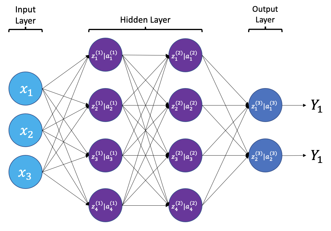
The smallest building block of a neural network is a single neuron. A typical neuron receives inputs (x1, x2, x3) which are multiplied by learnable weights (w1, w2, w3), then summed with a bias term (b). An activation function (f) determines the neuron output.
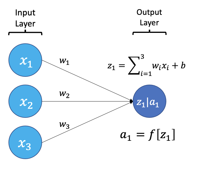
From a high level, a neural network is a system that takes input values in an “input layer”, processes these values with a collection of functions in one or more “hidden layers”, and then generates an output such as a prediction. The network has parameters that are systematically tweaked to allow pattern recognition.
 {a;t=“A simple neural
network with input, output, and 2 hidden layers”}
{a;t=“A simple neural
network with input, output, and 2 hidden layers”}
The layers shown in the network above are “dense” or “fully connected”. Each neuron is connected to all neurons in the preceeding layer. Dense layers are a common building block in neural network architectures.
“Deep learning” is an increasingly popular term used to describe certain types of neural network. When people talk about deep learning they are typically referring to more complex network designs, often with a large number of hidden layers.
Activation Functions
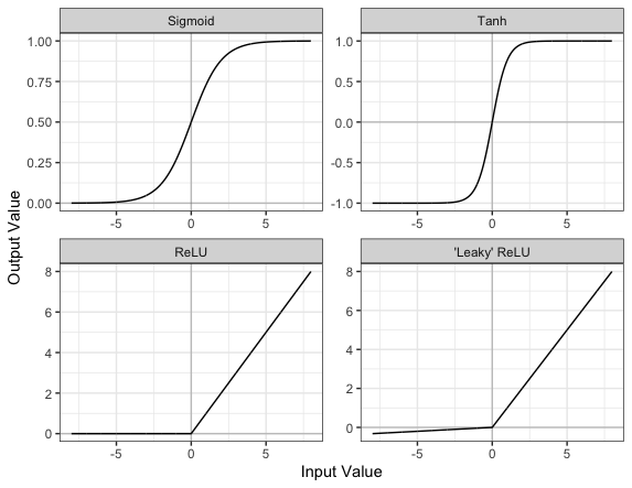
Part of the concept of a neural network is that each neuron can either be ‘active’ or ‘inactive’. This notion of activity and inactivity is attempted to be replicated by so called activation functions. The original activation function was the sigmoid function (related to its use in logistic regression). This would make each neuron’s activation some number between 0 and 1, with the idea that 0 was ‘inactive’ and 1 was ‘active’.
As time went on, different activation functions were used. For example the tanh function (hyperbolic tangent function), where the idea is a neuron can be active in both a positive capacity (close to 1), a negative capacity (close to -1) or can be inactive (close to 0).
The problem with both of these is that they suffered from a problem called model saturation. This is where very high or very low values are put into the activation function, where the gradient of the line is almost flat. This leads to very slow learning rates (it can take a long time to train models with these activation functions).
Another very popular activation function that tries to tackle this is the rectified linear unit (ReLU) function. This has 0 if the input is negative (inactive) and just gives back the input if it is positive (a measure of how active it is - the metaphor gets rather stretched here). This is much faster at training and gives very good performance, but still suffers model saturation on the negative side. Researchers have tried to get round this with functions like ‘leaky’ ReLU, where instead of returning 0, negative inputs are multiplied by a very small number.
Convolutional neural networks
Convolutional neural networks (CNNs) are a type of neural network that especially popular for vision tasks such as image recognition. CNNs are very similar to ordinary neural networks, but they have characteristics that make them well suited to image processing.
Just like other neural networks, a CNN typically consists of an input layer, hidden layers and an output layer. The layers of “neurons” have learnable weights and biases, just like other networks.
What makes CNNs special? The name stems from the fact that the architecture includes one or more convolutional layers. These layers apply a mathematical operation called a “convolution” to extract features from arrays such as images.
In a convolutional layer, a matrix of values referred to as a “filter” or “kernel” slides across the input matrix (in our case, an image). As it slides, values are multiplied to generate a new set of values referred to as a “feature map” or “activation map”.
Filters provide a mechanism for emphasising aspects of an input image. For example, a filter may emphasise object edges. See setosa.io for a visual demonstration of the effect of different filters.
Creating a convolutional neural network
Before training a convolutional neural network, we will first need to define the architecture. We can do this using the Keras and Tensorflow libraries.
PYTHON
# Create the architecture of our convolutional neural network, using
# the tensorflow library
from tensorflow.random import set_seed
from tensorflow.keras.layers import Dense, Dropout, Conv2D, MaxPool2D, Input, GlobalAveragePooling2D
from tensorflow.keras.models import Model

# set random seed for reproducibility
set_seed(42)

# Our input layer should match the input shape of our images.
# A CNN takes tensors of shape (image_height, image_width, color_channels)
# We ignore the batch size when describing the input layer
# Our input images are 256 by 256, plus a single colour channel.
inputs = Input(shape=(256, 256, 1))

# Let's add the first convolutional layer
x = Conv2D(filters=8, kernel_size=3, padding='same', activation='relu')(inputs)

# MaxPool layers are similar to convolution layers.
# The pooling operation involves sliding a two-dimensional filter over each channel of feature map and selecting the max values.
# We do this to reduce the dimensions of the feature maps, helping to limit the amount of computation done by the network.
x = MaxPool2D()(x)

# We will add more convolutional layers, followed by MaxPool
x = Conv2D(filters=8, kernel_size=3, padding='same', activation='relu')(x)
x = MaxPool2D()(x)
x = Conv2D(filters=12, kernel_size=3, padding='same', activation='relu')(x)
x = MaxPool2D()(x)
x = Conv2D(filters=12, kernel_size=3, padding='same', activation='relu')(x)
x = MaxPool2D()(x)
x = Conv2D(filters=20, kernel_size=5, padding='same', activation='relu')(x)
x = MaxPool2D()(x)
x = Conv2D(filters=20, kernel_size=5, padding='same', activation='relu')(x)
x = MaxPool2D()(x)
x = Conv2D(filters=50, kernel_size=5, padding='same', activation='relu')(x)

# Global max pooling reduces dimensions back to the input size
x = GlobalAveragePooling2D()(x)

# Finally we will add two "dense" or "fully connected layers".
# Dense layers help with the classification task, after features are extracted.
x = Dense(128, activation='relu')(x)

# Dropout is a technique to help prevent overfitting that involves deleting neurons.
x = Dropout(0.6)(x)

x = Dense(32, activation='relu')(x)

# Our final dense layer has a single output to match the output classes.
# If we had multi-classes we would match this number to the number of classes.
outputs = Dense(1, activation='sigmoid')(x)

# Finally, we will define our network with the input and output of the network
model = Model(inputs=inputs, outputs=outputs)
We can view the architecture of the model:
OUTPUT
Model: "model_39"
_________________________________________________________________
 Layer (type)                Output Shape              Param #
=================================================================
 input_9 (InputLayer)        [(None, 256, 256, 1)]     0

 conv2d_59 (Conv2D)          (None, 256, 256, 8)       80

 max_pooling2d_50 (MaxPoolin  (None, 128, 128, 8)      0
 g2D)

 conv2d_60 (Conv2D)          (None, 128, 128, 8)       584

 max_pooling2d_51 (MaxPoolin  (None, 64, 64, 8)        0
 g2D)

 conv2d_61 (Conv2D)          (None, 64, 64, 12)        876

 max_pooling2d_52 (MaxPoolin  (None, 32, 32, 12)       0
 g2D)

 conv2d_62 (Conv2D)          (None, 32, 32, 12)        1308

 max_pooling2d_53 (MaxPoolin  (None, 16, 16, 12)       0
 g2D)

 conv2d_63 (Conv2D)          (None, 16, 16, 20)        6020

 max_pooling2d_54 (MaxPoolin  (None, 8, 8, 20)         0
 g2D)

 conv2d_64 (Conv2D)          (None, 8, 8, 20)          10020

 max_pooling2d_55 (MaxPoolin  (None, 4, 4, 20)         0
 g2D)

 conv2d_65 (Conv2D)          (None, 4, 4, 50)          25050

 global_average_pooling2d_8   (None, 50)               0
 (GlobalAveragePooling2D)

 dense_26 (Dense)            (None, 128)               6528

 dropout_8 (Dropout)         (None, 128)               0

 dense_27 (Dense)            (None, 32)                4128

 dense_28 (Dense)            (None, 1)                 33

=================================================================
Total params: 54,627
Trainable params: 54,627
Non-trainable params: 0
_________________________________________________________________
MATLAB
Plotting
The mathematician Richard Hamming once said, “The purpose of computing is insight, not numbers,” and the best way to develop insight is often to visualize data. Visualization deserves an entire lecture (or course) of its own, but we can explore a few features of MATLAB here.
We will start by exploring the function plot. The most
common usage is to provide two vectors, like plot(X,Y).
Lets start by plotting the the average (accross patients) inflammation
over time. For the Y vector we can provide
per_day_mean, and for the X vector we can
simply use the day number, which we can generate as a range with
1:40. Then our plot can be generated with:
Callout
Note: If we only provide a vector as an argument it
plots a data-point for each value on the y axis, and it uses the index
of each element as the x axis. For our patient data the indices coincide
with the day of the study, so plot(per_day_mean) generates
the same plot. In most cases, however, using the indices on the x axis
is not desireable.
Callout
Note: We do not even need to have the vactor saved
as a variable. We would obtain the same plot with the command
plot(mean(patient_data, 1)).
As it is, the image is not very informative. We need to give the
figure a title and label the axes using xlabel
and ylabel, so that other people can understand what it
shows (including us if we return to this plot 6 months from now).
Much better, now the image actually communicates something.
The result is roughly a linear rise and fall, which is suspicious: based on other studies, we expect a sharper rise and slower fall. Let’s have a look at two other statistics: the maximum and minimum inflammation per day across all patients.
MATLAB
>> plot(per_day_max)
>> title('Maximum inflammation per day')
>> ylabel('Inflammation')
>> xlabel('Day of trial')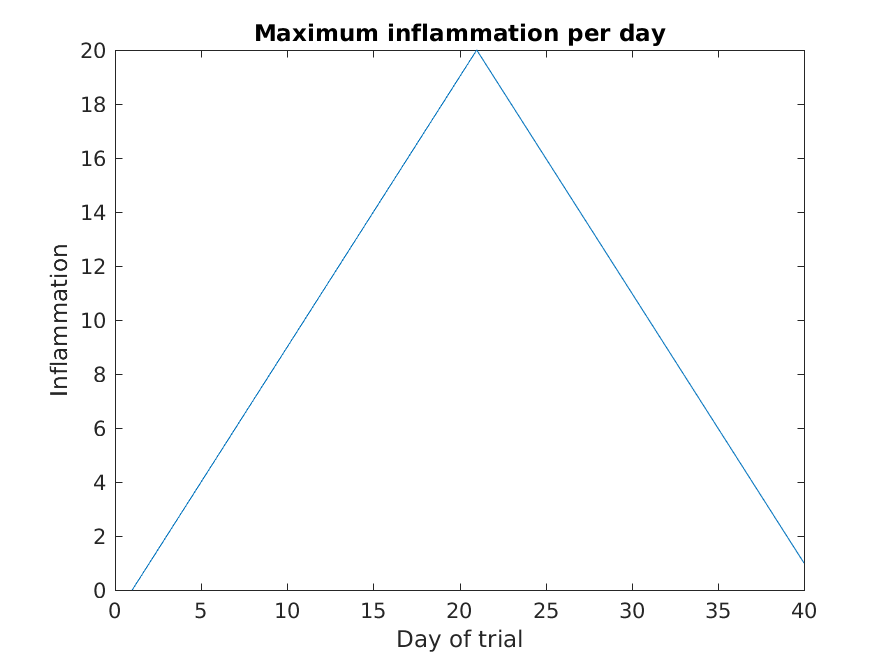
MATLAB
>> plot(per_day_min)
>> title('Minimum inflammation per day')
>> ylabel('Inflammation')
>> xlabel('Day of trial')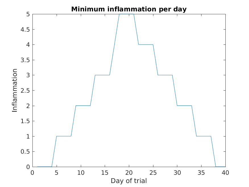
From the figures, we see that the maximum value rises and falls perfectly smoothly, while the minimum seems to be a step function. Neither result seems particularly likely, so either there’s a mistake in our calculations or something is wrong with our data.
Multiple lines in a plot
It is often the case that we want more than one line in a single
plot. In matlab we can “hold” a plot and keep plotting on top. For
example, we might want to contrast the mean values accross patients with
the information of a single patient. If we are displaying more than one
line, it is important we add a legend. We can specify the legend names
by adding ,'DisplayName',"legend name here" inside the plot
function. We then need to activate the legend by running
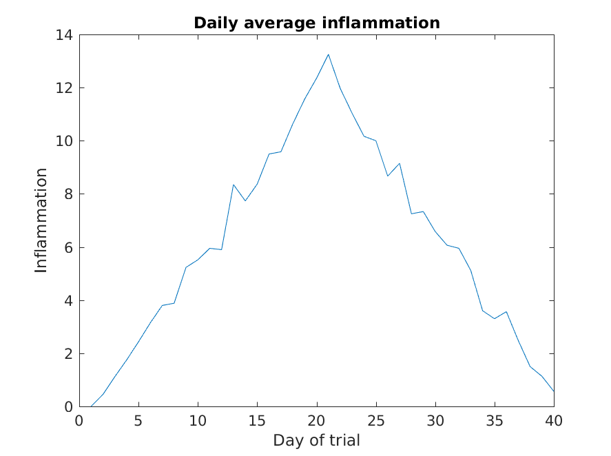
legend So, to plot the mean values we first do:
MATLAB
>> plot(per_day_mean,'DisplayName',"Mean")
>> legend
>> title('Daily average inflammation')
>> xlabel('Day of trial')
>> ylabel('Inflammation')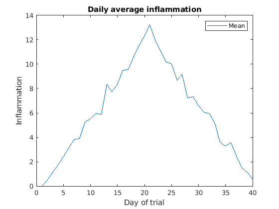
Then, we can use the instruction hold on to add a plot
for patient_5.
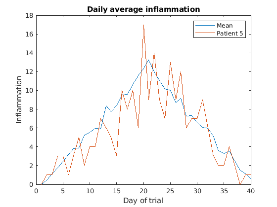
Remember to tell matlab you are done by adding hold off
when you are done!
Subplots
It is often convenient to combine multiple plots into one figure. The
subplot(m,n,p)command allows us to do just that. The first
two parameter define a grid of m rows and n
columns, in which our plots will be placed. The third parameter
indicates the position on the grid that we want to use for the “next”
plot command. For example, we can show the average daily min and max
plots together with:
MATLAB
>> subplot(1, 2, 1)
>> plot(per_day_max)
>> ylabel('max')
>> xlabel('day')

>> subplot(1, 2, 2)
>> plot(per_day_min)
>> ylabel('min')
>> xlabel('day')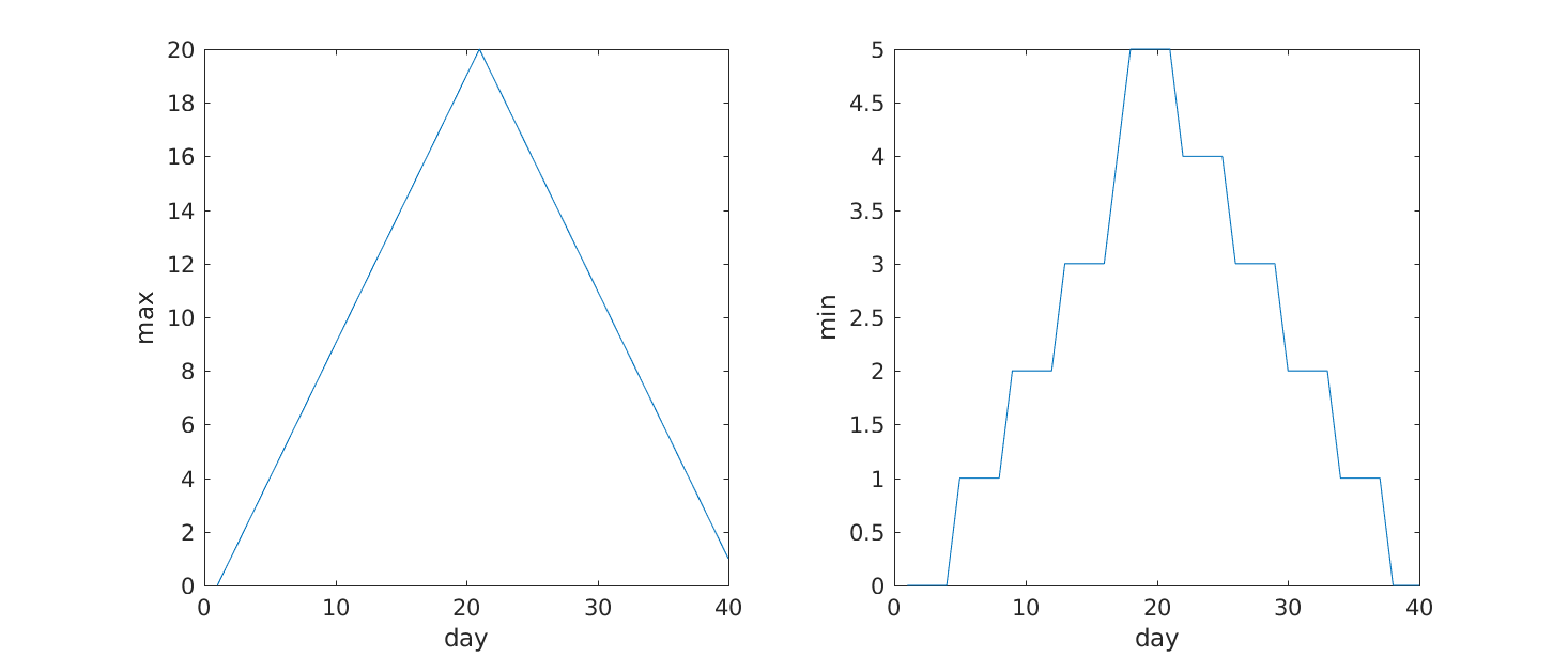
Heatmaps
If we wanted to look at all our data at the same time we need a three dimensions: One for the patients, one for the days, and another one for the inflamation values. An option is to use a heatmap, that is, use the colour of each point to represent the inflamation values.
In matlab, at least two methods can do this for us. The heatmap
function takes a table as input and produces a heatmap:
MATLAB
>> heatmap(patient_data)
>> title('Inflammation')
>> xlabel('Day of trial')
>> ylabel('Patient number')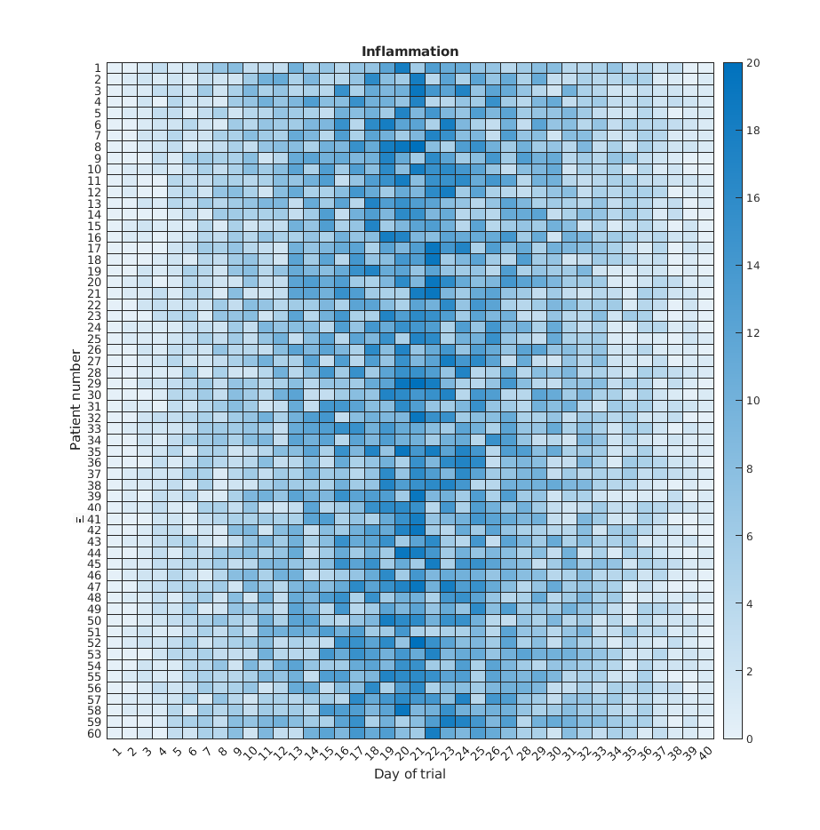
We gain something by visualizing the whole dataset at once, but it is harder to distinwish the overly linear rises and fall over a 40 day period.
Similarly, the imagesc
function represents the matrix as a color image.
MATLAB
>> imagesc(patient_data)
>> title('Inflammation')
>> xlabel('Day of trial')
>> ylabel('Patient number')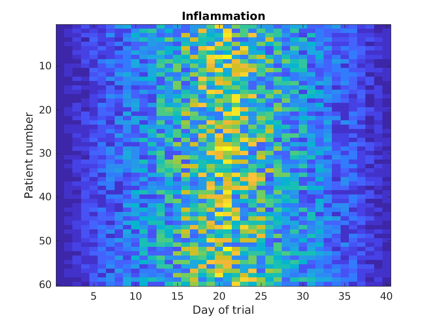
Every value in the matrix is mapped to a color. Blue regions in this heat map are low values, while yellow shows high values.
Both functions provide very similar information, and can be tweaked
to your liking. The imagesc function is usually only used
for purely numerical arrays, whereas heatmap can process tables
(that can have strings or categories in them). In our case, which one
you use is a matter of taste.
Is all our data corrupt?
Our work so far has convinced us that something is wrong with our first data file. We would like to check the other 11 the same way, but typing in the same commands repeatedly is tedious and error-prone. Since computers don’t get bored (that we know of), we should create a way to do a complete analysis with a single command, and then figure out how to repeat that step once for each file. These operations are the subjects of the next two lessons.
Content from Writing MATLAB Scripts
Last updated on 2023-08-21 | Edit this page
Overview
Questions
- “How can I save and re-use my programs?”
Objectives
- “Write and save MATLAB scripts.”
- “Save MATLAB plots to disk.”
So far, we’ve typed in commands one-by-one on the command line to get MATLAB to do things for us. But what if we want to repeat our analysis? Sure, it’s only a handful of commands, and typing them in shouldn’t take us more than a few minutes. But if we forget a step or make a mistake, we’ll waste time rewriting commands. Also, we’ll quickly find ourselves doing more complex analyses, and we’ll need our results to be more easily reproducible.
In addition to running MATLAB commands one-by-one on the command
line, we can also write several commands in a script. A MATLAB
script is just a text file with a .m extension. We’ve
written commands to load data from a .csv file, compute
statistics of the data and display some plots about that data. Let’s put
those commands in a script called patient_analysis.m, which
we’ll save in the src directory in our current
folder,matlab-novice-inflammation.
To create a new script we can click the “New script” button on the top left, or use the command:
Matlab will create a file called patient_analysis.m in
the src folder. It is important that we let matlab know
that we want it to find stuff in this folder. To do this, right click on
the folder icon in the file browser and select “Add to Path”.
The MATLAB path
MATLAB knows about files in the current directory, but if we want to run a script saved in a different location, we need to make sure that this file is visible to MATLAB. We do this by adding directories to the MATLAB path. The path is a list of directories MATLAB will search through to locate files.
To add a directory to the MATLAB path, we go to the Home
tab, click on Set Path, and then on
Add with Subfolders.... We navigate to the directory and
add it to the path to tell MATLAB where to look for our files. When you
refer to a file (either code or data), MATLAB will search all the
directories in the path to find it. Alternatively, for data files, we
can provide the relative or absolute file path.
GNU Octave
Octave has only recently gained a MATLAB-like user interface. To
change the path in any version of Octave, including command-line-only
installations, use addpath('path/to/directory')
We can now type the contents of the script:
MATLAB
% Load patient data
patient_data = readmatrix('data/inflammation-01.csv');

% Compute global statistics
g_mean = mean(patient_data(:));
g_max = max(patient_data(:));
g_min = min(patient_data(:));

% Compute patient statistics
p_mean = mean(patient_data(5,:));
p_max = max(patient_data(5,:));
p_min = min(patient_data(5,:));

% Compare patient vs global
disp('Patient 5:')
disp('High mean?')
disp(p_mean > g_mean)
disp('Highest max?')
disp(p_max == g_max)
disp('Lowest min?')
disp(p_min == g_min)
Now, before running this script lets clear our workplace so that we can see what is happening.
If you now run the script by clicking “Run” on the graphical user
interface, pressing F5 on the keyboard, or typing the
script’s name patient_analysis on the command line (without
extention), you’ll see a bunch of variables appear on the workspace and
this output:
OUTPUT
Patient 5:
High mean?
   0
Highest max?
   0
Lowest min?
   1
Remember, we supressed most outputs with ;, so the only
lines printed are the ones with disp.
As you can see, the script ran every line of code in the script in
order, and created any variable we asked for. Having the code in the
script makes it much easier to follow what we are doing, and also make
changes. For example, if we now want to look at patient 8, all we need
to do is change the number in lines 10, 11 and 12. We can actually do a
bit better, and replace that number for a variable
patient_number. This variable needs to exist before it is
used, so lets insert it before computing the patient statistics, like
so:
MATLAB
% Load patient data
patient_data = readmatrix('data/inflammation-01.csv');

% Compute global statistics
g_mean = mean(patient_data(:));
g_max = max(patient_data(:));
g_min = min(patient_data(:));

patient_number = 8;

% Compute patient statistics
p_mean = mean(patient_data(patient_number,:));
p_max = max(patient_data(patient_number,:));
p_min = min(patient_data(patient_number,:));

% Compare patient vs global
disp('Patient:')
disp(patient_number)
disp('High mean?')
disp(p_mean > g_mean)
disp('Highest max?')
disp(p_max == g_max)
disp('Lowest min?')
disp(p_min == g_min)
Note that we also changed the disp commands to show the right patient number.
Getting the results for whichever patient is now as simple as
changing the value of patient_number.
For the case of patient 8, we get:
OUTPUT
Patient 8:
High mean?
   1
Highest max?
   1
Lowest min?
   1
Help text
You might have noticed that we described what we want our code to do
using the percent sign: %. This is another plus of writing
scripts: you can comment your code to make it easier to understand when
you come back to it after a while.
A comment can appear on any line, but be aware that the first line or
block of comments in a script or function is used by MATLAB as the
help text. When we use the help command,
MATLAB returns the help text. The first help text line (known
as the H1 line) typically includes the name of the
program, and a brief description. The help command works in
just the same way for our own programs as for built-in MATLAB functions.
You should write help text for all of your own scripts and
functions.
Let’s write an H1 line at the top of our script:
MATLAB
% PATIENT_ANALYSIS Computes mean, max and min of a patient and compares to global statistics.We can then get help for our script by running
OUTPUT
patient_analysis Computes mean, max and min of a patient and compares to global statistics.Script for plotting
Of course, our scripts can be as complicated as we like. There were a lot of commands involved with plotting, so lets try and put that in a script.
Create a new script in the current directory called
plot_daily_average.m
In the script, lets recap what we need to do:
MATLAB
% PLOT_DAILY_AVERAGE   Plots daily average inflammation accross patients.

% Load patient data
patient_data = readmatrix('data/inflammation-01.csv');

figure

% Plot average inflammation per day
plot(mean(patient_data, 1))
title('Daily average inflammation')
xlabel('Day of trial')
ylabel('Inflammation')
Note that we are explicitly creating a new figure window using the
figure command.
Try this on the command line:
MATLAB’s plotting commands only create a new figure window if one doesn’t already exist: the default behaviour is to reuse the current figure window as we saw in the previous episode. Explicitly creating a new figure window in the script avoids any unexpected results from plotting on top of existing figures.
Now lets run the script:
You should see the figure appear.
Let’s modify our plot_daily_average script so that it
creates sub-plots, rather than individual plots.
MATLAB
% PLOT_DAILY_AVERAGE   Plots daily average, max and min inflammation accross patients.

% Load patient data
patient_data = readmatrix('data/inflammation-01.csv');

figure

% Plot average inflammation per day
subplot(1, 3, 1)
plot(mean(patient_data, 1))
title('Daily average inflammation')
xlabel('Day of trial')
ylabel('Inflammation')

% Plot max inflammation per day
subplot(1, 3, 2)
plot(max(patient_data, [], 1))
title('Max')
ylabel('Inflammation')
xlabel('Day of trial')

% Plot min inflammation per day
subplot(1, 3, 3)
plot(min(patient_data, [], 1))
title('Min')
ylabel('Inflammation')
xlabel('Day of trial')
The script now allows us to create all 3 plots with a single command:
plot_daily_average.
We can ask matlab to save the image too using the print
command. In order to maintain an organised project we’ll save the images
in the results directory:
Callout
Note:
If you have a printer configured on your computer the
print command may send it to the printer. You can instead
use saveas, which requiere two arguments: a figure and a
filename. You can get the current figure with gcf, and
specify the filename with an extension, like so:
When saving plots to disk, it’s sometimes useful to turn off their visibility as MATLAB plots them. For example, we might not want to view (or spend time closing) the figures in MATLAB, and not displaying the figures could make the script run faster.
Let’s add a couple of lines of code to do this.
We can ask MATLAB to create an empty figure window without displaying
it by setting its 'visible' property to 'off',
like so:
When we do this, we have to be careful to manually “close” the figure after we are doing plotting on it - the same as we would “close” an actual figure window if it were open:
Adding these two lines, our finished script looks like this:
MATLAB
% PLOT_DAILY_AVERAGE Saves plot of daily average, max and min inflammation accross patients.
% Load patient data
patient_data = readmatrix('data/inflammation-01.csv');
figure('visible', 'off')
% Plot average inflammation per day
subplot(1, 3, 1)
plot(mean(patient_data, 1))
title('Daily average inflammation')
xlabel('Day of trial')
ylabel('Inflammation')
% Plot max inflammation per day
subplot(1, 3, 2)
plot(max(patient_data, [], 1))
title('Max')
ylabel('Inflammation')
xlabel('Day of trial')
% Plot min inflammation per day
subplot(1, 3, 3)
plot(min(patient_data, [], 1))
title('Min')
ylabel('Inflammation')
xlabel('Day of trial')
% Save plot in 'results' folder as png image:
saveas(gcf,'results/daily_average_01.png')
close()The scripts we’ve written make regenerating plots easier, and looking at individual patient’s data much simpler, but we still need to open the script, change the patient number, save, and run. In contrast, when we have used functions we can provide arguments, which are then used to do something. So, can we create our own functions?
Key Points
- “Save MATLAB code in files with a
.msuffix.”
Content from Creating Functions
Last updated on 2023-08-21 | Edit this page
Overview
Questions
- “How can I teach MATLAB how to do new things?”
Objectives
- “Compare and contrast MATLAB function files with MATLAB scripts.”
- “Define a function that takes arguments.”
- “Test a function.”
- “Recognize why we should divide programs into small, single-purpose functions.”
In the patient_analysis script we created, we can choose
which patient to analyse by modifying the variable
patient_number. If we want patient 13, we need to open
patient_analysis.m, go to line 9, modify the variable, save
and then run patient_analysis. This is a lot of steps for
such a simple request.
We have used a few predefined Matlab functions, to which we can provide arguments. So how can we define a function in Matlab?
A MATLAB function must be saved in a text file with a
.m extension. The name of that file must be the same as the
function defined inside it. The name must start with a letter and cannot
contain spaces.
The first line of our function is called the function
definition. Anything following the function definition line is
called the body of the function. The keyword end
marks the end of the function body, and the function won’t know about
any code after end.
A function can have multiple input and output parameters if required, but isn’t required to have any of either. The general form of a function is shown in the pseudo-code below:
MATLAB
function [out1, out2] = function_name(in1, in2)
    % FUNCTION_NAME   Function description
    %    Can add more text for the function help
    %    An example is always useful!

    % This section below is called the body of the function
    out1 = something calculated;
    out2 = something else;
end
Just as we saw with scripts, functions must be visible to MATLAB, i.e., a file containing a function has to be placed in a directory that MATLAB knows about. The most convenient of those directories is the current working directory.
GNU Octave
In common with MATLAB, Octave searches the current working directory and the path for functions called from the command line.
We already have a .m file called
patient_analysis, so lets define a function with that
name.
Open the patient_analysis.m file, if you don’t already
have it open. Instead of line 9, where patient_number is
set, we want to provide that variable as an input. So lets remove that
line, and right at the top of our script we’ll add the function
definition telling matlab what our function is called and what inputs it
needs.
MATLAB
function patient_analysis(patient_number)
    % PATIENT_ANALYSIS   Computes mean, max and min of a patient and compares to global statistics.
    %    Takes the patient number as an input, and prints the relevant information to console.
    %    Sample usage:
    %       patient_analysis(5)

    % Load patient data
    patient_data = readmatrix('data/inflammation-01.csv');

    % Compute global statistics
    g_mean = mean(patient_data(:));
    g_max = max(patient_data(:));
    g_min = min(patient_data(:));

    % Compute patient statistics
    p_mean = mean(patient_data(patient_number,:));
    p_max = max(patient_data(patient_number,:));
    p_min = min(patient_data(patient_number,:));

    % Compare patient vs global
    disp('Patient:')
    disp(patient_number)
    disp('High mean?')
    disp(p_mean > g_mean)
    disp('Highest max?')
    disp(p_max == g_max)
    disp('Lowest min?')
    disp(p_min == g_min)

end
Congratulations! You’ve now created a Matlab function.
You may have noticed that the code inside the function is indented. Matlab does not need this, but it makes it much more readable!
Lets clear our workspace and run our function in the command line:
OUTPUT
Patient 5:
High mean?
   1
Highest max?
   0
Lowest min?
   1
So now we can get the patient analysis of whichever patient we want,
and we do not need to modify patient_analysis.m anymore.
However, you may have noticed that we have no variables in our
workspace. Inside the function, the variables patient_data,
g_mean, g_max, g_min,
p_mean, p_max, and p_min are
created, but then they are deleted when the function ends.
This is one of the major differences between scripts and functions: a script can be thought of as automating the command line, with full access to all variables in the base workspace, whereas a function has its own separate workspace.
To be able to access variables from your workspace, you have to pass them in as inputs. To be able to save variables to your workspace, it needs to return them as outputs.
Lets say, for example, that we want to save the mean of each patient.
In our patient_analysis.m we already compute the value and
save it in p_mean, but we need to tell matlab that we want
the function to return it.
To do that we modify the function definition like this:
It is important that the variable name is the same that is used inside the function.
If we now run our function in the command line, we get:
OUTPUT
Patient 5:
High mean?
   1
Highest max?
   0
Lowest min?
   1

p13 =
    6.2250
We could return more outputs if we want. For example, lets return the min and max as well. To do that, we need to specify all the outputs in square brackets, as an array. So we need to replace the function definition for:
To call our function now we need to provide space for all 3 outputs, so in the command line, we run it as:
OUTPUT
Patient 5:
High mean?
   1
Highest max?
   0
Lowest min?
   1
p13_mean =
    6.2250
p13_max =
    17
p13_min =
     0
Callout
Note If you had not provided space for all the
outputs, Matlab assumes you are only interested in the first one, so
ans would save the mean.
Plotting daily average of different data files
Look back at the plot_daily_average script. The data and
resulting image file names are hard-coded in the script. We actually
have 12 datafiles. Turn the script into a function that lets you
generate the plots for any of the files.
The function should operate on a single data file, and should have
two parameters: data_file and plot_file. When
called, the function should create the three graphs, and save the plot
as plot_file.
You should mostly be reusing code from the plot_all
script.
MATLAB
function plot_daily_average(data_file,plot_name)
    %PLOT_DAILY_AVERAGE   Plots daily average, max and min inflammation accross patients.
    %   The function takes the data in data_file and saves it as plot_name
    %   Example usage:
    %       plot_daily_average('data/inflammation-03.csv','results/plot3.png')

    % Load patient data
    patient_data = readmatrix(data_file);

    figure('visible', 'off')

    % Plot average inflammation per day
    subplot(1, 3, 1)
    plot(mean(patient_data, 1))
    title('Daily average inflammation')
    xlabel('Day of trial')
    ylabel('Inflammation')

    % Plot max inflammation per day
    subplot(1, 3, 2)
    plot(max(patient_data, [], 1))
    title('Max')
    ylabel('Inflammation')
    xlabel('Day of trial')

    % Plot min inflammation per day
    subplot(1, 3, 3)
    plot(min(patient_data, [], 1))
    title('Min')
    ylabel('Inflammation')
    xlabel('Day of trial')

    % Save plot in 'results' folder as png image:
    saveas(gcf,plot_name)

    close()
end
Plotting patient vs mean
Create a function called patient_vs_mean that generates
a plot like this one:
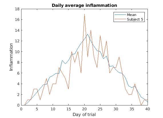
The function should have the following inputs:
per_day_mean- A 1D array with the average inflamation per day already loaded (you’ll have to load the data and compute per_day_mean before calling the function).pataient_data- A 1D array with the data for the patient of interest only.patient_reference- A string that will be used to identify the patient on the plot, and also as a file name (you should add the extensionpngin your function).
When called, the function should create and save the plot as
patient_reference.png in the results folder.
Look back at the previous lessons if you need to!
MATLAB
function patient_vs_mean(per_day_mean,pataient_data,patient_reference)
    % PATIENT_VS_MEAN   Plots the global mean and patient inflamation on top of each other.
    %   per_day_mean should be a vector with the global mean.
    %   pataient_data should be a vector with only the patient data.
    %   patient_reference will be used to identify the patient on the plot.
    %
    %   Sample usage:
    %       patient_data = readmatrix('data/inflammation-01.csv');
    %       per_day_mean = mean(patient_data);
    %       patient_vs_mean(per_day_mean,patient_data(5,:),"Subject 5")

    figure('visible', 'off')

    %Plot per_day_mean
    plot(per_day_mean,'DisplayName',"Mean")
    legend
    title('Daily average inflammation')
    xlabel('Day of trial')
    ylabel('Inflammation')

    %Overlap patient data
    hold on
    plot(pataient_data,'DisplayName',patient_reference)
    hold off

    % Save plot
    saveas(gcf,"results/"+patient_reference+".png")

    close()

end
Key Points
- “Break programs up into short, single-purpose functions with meaningful names.”
- “Define functions using the
functionkeyword.”
Content from Repeating With Loops
Last updated on 2023-08-21 | Edit this page
Overview
Questions
- “How can I repeat the same operations on multiple values?”
Objectives
- “Explain what a for loop does.”
- “Correctly write for loops that repeat simple commands.”
- “Trace changes to a loop variable as the loops runs.”
- “Use a for loop to process multiple files”
Recall that we have to do this analysis for every one of our dozen datasets, and we need a better way than typing out commands for each one, because we’ll find ourselves writing a lot of duplicate code. Remember, code that is repeated in two or more places will eventually be wrong in at least one. Also, if we make changes in the way we analyze our datasets, we have to introduce that change in every copy of our code. To avoid all of this repetition, we have to teach MATLAB to repeat our commands, and to do that, we have to learn how to write loops.
Suppose we want to print each character in the word “lead” on a line
of its own. One way is to use four disp statements:
MATLAB
%LOOP_DEMO   Demo script to explain loops

word = 'lead';

disp(word(1))
disp(word(2))
disp(word(3))
disp(word(4))
OUTPUT
l
e
a
d
But this is a bad approach for two reasons:
It doesn’t scale: if we want to print the characters in a string that’s hundreds of letters long, we’d be better off typing them in.
It’s fragile: if we change
wordto a longer string, it only prints part of the data, and if we change it to a shorter one, it produces an error, because we’re asking for characters that don’t exist.
MATLAB
%LOOP_DEMO   Demo script to explain loops

word = 'tin';

disp(word(1))
disp(word(2))
disp(word(3))
disp(word(4))
error: A(I): index out of bounds; value 4 out of bound 3{: .error}
There’s a better approach:
MATLAB
%LOOP_DEMO   Demo script to explain loops

word = 'lead';

for letter = 1:4
    disp(word(letter))
end
OUTPUT
l
e
a
d
This improved version uses a for loop to repeat an operation—in this case, printing to the screen—once for each element in an array.
The general form of a for loop is:
for variable = collection
    do things with variable
end
{: .source}
The for loop executes the commands in the loop
body for every value in the array collection. This
value is called the loop
variable, and we can call it whatever we like. In our example, we
gave it the name letter.
We have to terminate the loop body with the end keyword,
and we can have as many commands as we like in the loop body. But, we
have to remember that they will all be repeated as many times as there
are values in collection.
Our for loop has made our code more scalable, and less fragile. There’s still one little thing about it that should bother us. For our loop to deal appropriately with shorter or longer words, we have to change the first line of our loop by hand:
MATLAB
%LOOP_DEMO   Demo script to explain loops

word = 'tin';

for letter = 1:3
    disp(word(letter))
end
OUTPUT
t
i
n
Although this works, it’s not the best way to write our loop:
We might update
wordand forget to modify the loop to reflect that change.We might make a mistake while counting the number of letters in
word.
Fortunately, MATLAB provides us with a convenient function to write a better loop:
MATLAB
%LOOP_DEMO   Demo script to explain loops

word = 'aluminum';

for letter = 1:length(word)
    disp(word(letter))
end
OUTPUT
a
l
u
m
i
n
u
m
This is much more robust code, as it can deal identically with words of arbitrary length. Loops are not only for working with strings, they allow us to do repetitive calculations regardless of data type. Here’s another loop that calculates the sum of all even numbers between 1 and 10:
MATLAB
%LOOP_DEMO   Demo script to explain loops

total = 0;
for even_number = 2 : 2 : 10
    total = total + even_number;
end

disp('The sum of all even numbers between 1 and 10 is:')
disp(total)
It’s worth tracing the execution of this little program step by step.
The debugger
We can use the MATLAB debugger to trace the execution of a program.
The first step is to set a break point by clicking
just to the right of a line number on the - symbol. A red
circle will appear — this is the break point, and when we run the
script, MATLAB will pause execution at that line.
A green arrow appears, pointing to the next line to be run. To
continue running the program one line at a time, we use the
step button.
We can then inspect variables in the workspace or by hovering the
cursor over where they appear in the code, or get MATLAB to evaluate
expressions in the command window (notice the prompt changes to
K>>).
This process is useful to check your understanding of a program, in order to correct mistakes.
This process is illustrated below: 
Since we want to sum only even numbers, the loop index
even_number starts at 2 and increases by 2 with every
iteration. When we enter the loop, total is zero - the
value assigned to it beforehand. The first time through, the loop body
adds the value of the first even number (2) to the old value of
total (0), and updates total to refer to that
new value. On the next loop iteration, even_number is 4 and
the initial value of total is 2, so the new value assigned
to total is 6. After even_number reaches the
final value (10), total is 30; since this is the end of the
range for even_number the loop finishes and the
disp statements give us the final answer.
Note that a loop variable is just a variable that’s being used to record progress in a loop. It still exists after the loop is over, and we can re-use variables previously defined as loop variables as well:
OUTPUT
10Performing Exponentiation
MATLAB uses the caret (^) to perform exponentiation:
OUTPUT
125You can also use a loop to perform exponentiation. Remember that
b^x is just b*b*b*… x times.
Let a variable b be the base of the number and
x the exponent. Write a loop to compute b^x.
Check your result for b = 4 and x = 5.
Incrementing with Loops
Write a loop that spells the word “aluminum,” adding one letter at a time:
OUTPUT
a
al
alu
alum
alumi
alumin
aluminu
aluminumLooping in Reverse
In MATLAB, the colon operator (:) accepts a stride or
skip argument between the start and stop:
OUTPUT
1 4 7 10OUTPUT
11 8 5 2Using this, write a loop to print the letters of “aluminum” in reverse order, one letter per line.
OUTPUT
m
u
n
i
m
u
l
aAnalyzing patient data from multiple files
We now have almost everything we need to process multiple data files
using a loop and the plotting code in our plot_patient1
script.
We still need to generate a list of data files to process, and then we can use a loop to repeat the analysis for each file.
We can use the dir command to return a structure
array containing the names of the files in the
data directory. Each element in this structure
array is a structure, containing information about
a single file in the form of named fields.
OUTPUT
files =
  12×1 struct array with fields:
    name
    folder
    date
    bytes
    isdir
    datenum
To access the name field of the first file, we can use the following syntax:
OUTPUT
inflammation-01.csvTo get the modification date of the third file, we can do:
OUTPUT
26-Jul-2015 22:24:31A good first step towards processing multiple files is to write a
loop which prints the name of each of our files. Let’s write this in a
script plot_all.m which we will then develop further:
MATLAB
%PLOT_ALL	Developing code to automate inflammation analysis

files = dir('data/inflammation-*.csv');

for i = 1:length(files)
	file_name = files(i).name;
	disp(file_name)
endOUTPUT
inflammation-01.csv
inflammation-02.csv
inflammation-03.csv
inflammation-04.csv
inflammation-05.csv
inflammation-06.csv
inflammation-07.csv
inflammation-08.csv
inflammation-09.csv
inflammation-10.csv
inflammation-11.csv
inflammation-12.csv
Another task is to generate the file names for the figures we’re
going to save. Let’s name the output file after the data file used to
generate the figure. So for the data set
inflammation-01.csv we will call the figure
inflammation-01.png. We can use the replace
command for this purpose.
The syntax for the replace command is like this:
So for example if we have the string big_shark and want
to get the string little_shark, we can execute the
following command:
OUTPUT
little_sharkRecall that we’re saving our figures to the results
directory. The best way to generate a path to a file in MATLAB is by
using the fullfile command. This generates a file path with
the correct separators for the platform you’re using (i.e. forward slash
for Linux and macOS, and backslash for Windows). This makes your code
more portable which is great for collaboration.
Putting these concepts together, we can now generate the paths for the data files, and the image files we want to save:
MATLAB
%PLOT_ALL	Developing code to automate inflammation analysis

files = dir('data/inflammation-*.csv');

for i = 1:length(files)
    file_name = files(i).name;

    % Generate string for image name
    img_name = replace(file_name, '.csv', '.png');

    % Generate path to data file and image file
    file_name = fullfile('data', file_name);
    img_name = fullfile('results',img_name);

    disp(file_name)
    disp(img_name)
end
OUTPUT
data/inflammation-01.csv
results/inflammation-01.png
data/inflammation-02.csv
results/inflammation-02.png
data/inflammation-03.csv
results/inflammation-03.png
data/inflammation-04.csv
results/inflammation-04.png
data/inflammation-05.csv
results/inflammation-05.png
data/inflammation-06.csv
results/inflammation-06.png
data/inflammation-07.csv
results/inflammation-07.png
data/inflammation-08.csv
results/inflammation-08.png
data/inflammation-09.csv
results/inflammation-09.png
data/inflammation-10.csv
results/inflammation-10.png
data/inflammation-11.csv
results/inflammation-11.png
data/inflammation-12.csv
results/inflammation-12.png
We’re now ready to modify plot_all.m to actually process
multiple data files:
MATLAB
%PLOT_ALL   Print statistics for all patients.
%           Save plots of statistics to disk.

files = dir('data/inflammation-*.csv');

% Process each file in turn
for i = 1:length(files)
    file_name = files(i).name;

    % Generate strings for image names:
    img_name  = replace(file_name, '.csv', '.png');

    % Generate path to data file and image file
    file_name = fullfile('data', file_name);
    img_name  = fullfile('results', img_name);

    patient_data = readmatrix(file_name);

    % Create figures
    figure('visible', 'off')

    subplot(2, 2, 1)
    plot(mean(patient_data, 1))
    title('Average')
    ylabel('Inflammation')
    xlabel('Day')

    subplot(2, 2, 2)
    plot(max(patient_data, [], 1))
    title('Max')
    ylabel('Inflammation')
    xlabel('Day')

    subplot(2, 2, 3)
    plot(min(patient_data, [], 1))
    title('Min')
    ylabel('Inflammation')
    xlabel('Day')

    print(img_name, '-dpng')
    close()
end
We run the modified script using its name in the Command Window:
The first three figures output to the results directory
are as shown below:
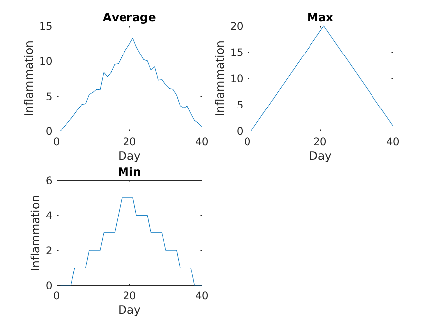
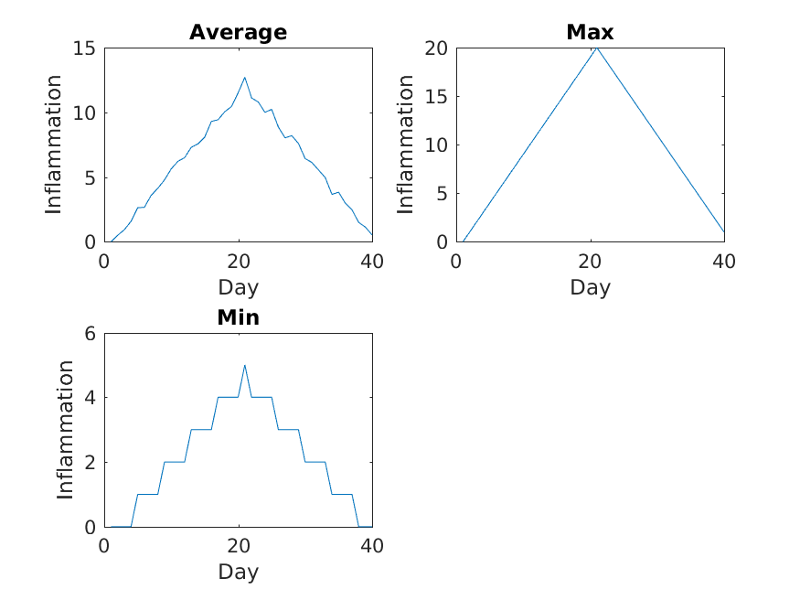

Sure enough, the maxima of these data sets show exactly the same ramp as the first, and their minima show the same staircase structure.
We’ve now automated the analysis and have confirmed that all the data files we have looked at show the same artifact. This is what we set out to test, and now we can just call one script to do it. With minor modifications, this script could be re-used to check all our future data files.
Key Points
- “Use
forto create a loop that repeats one or more operations.”
Content from Making Choices
Last updated on 2023-08-21 | Edit this page
Overview
Questions
- “How can programs do different things for different data values?” objectives:
- “Construct a conditional statement using if, elseif, and else”
- “Test for equality within a conditional statement”
- “Combine conditional tests using AND and OR”
- “Build a nested loop”
Objectives
- xxx
Our previous lessons have shown us how to manipulate data and repeat things. However, the programs we have written so far always do the same things, regardless of what data they’re given. We want programs to make choices based on the values they are manipulating.
The tool that MATLAB gives us for doing this is called a conditional statement, and it looks like this:
OUTPUT
not greater
done
The second line of this code uses the keyword if to tell
MATLAB that we want to make a choice. If the test that follows is true,
the body of the if (i.e., the lines between if
and else) are executed. If the test is false, the body of
the else (i.e., the lines between else and
end) are executed instead. Only one or the other is ever
executed.
Conditional statements don’t have to have an else block.
If there isn’t one, MATLAB simply doesn’t do anything if the test is
false:
MATLAB
num = 53;
disp('before conditional...')

if num > 100
    disp('53 is greater than 100')
end

disp('...after conditional')
OUTPUT
before conditional...
...after conditional
We can also chain several tests together using elseif.
This makes it simple to write a script that gives the sign of a
number:
MATLAB
%CONDITIONAL_DEMO   Demo script to illustrate use of conditionals

num = 53;

if num > 0
    disp('num is positive')
elseif num == 0
    disp('num is zero')
else
    disp('num is negative')
end
One important thing to notice in the code above is that we use a
double equals sign == to test for equality rather than a
single equals sign. This is because the latter is used to mean
assignment. In our test, we want to check for the equality of
num and 0, not assign 0 to
num. This convention was inherited from C, and it does take
a bit of getting used to…
During a conditional statement, if one of the conditions is true, this marks the end of the test: no subsequent conditions will be tested and execution jumps to the end of the conditional.
Let’s demonstrate this by adding another condition which is true.
MATLAB
% Demo script to illustrate use of conditionals
num = 53;

if num > 0
    disp('num is positive')
elseif num == 0
    disp('num is zero')
elseif num > 50
    % This block will never be executed
    disp('num is greater than 50')
else
    disp('num is negative')
end
We can also combine tests, using && (and) and
|| (or). && is true if both tests are
true:
OUTPUT
one part is not true|| is true if either test is true:
OUTPUT
at least one part is trueIn this case, “either” means “either or both”, not “either one or the other but not both”.
True and False Statements
The conditions we have tested above evaluate to a logical value:
true or false. However these numerical
comparison tests aren’t the only values which are true or
false in MATLAB. For example, 1 is considered
true and 0 is considered false.
In fact, any value can be used in a conditional statement.
Run the code below in order to discover which values are considered
true and which are considered false.
MATLAB
if ''
    disp('empty string is true')
else
    disp('empty string is false')
end

if 'foo'
    disp('non empty string is true')
else
    disp('non empty string is false')
end

if []
    disp('empty array is true')
else
    disp('empty array is false')
end

if [22.5, 1.0]
    disp('non empty array is true')
else
    disp('non empty array is false')
end

if [0, 0]
    disp('array of zeros is true')
else
    disp('array of zeros is false')
end

if true
    disp('true is true')
else
    disp('true is false')
end
Close Enough
Write a script called near that performs a test on two
variables, and displays 1 when the first variable is within
10% of the other and 0 otherwise. Compare your
implementation with your partner’s: do you get the same answer for all
possible pairs of numbers?
Another thing to realize is that if statements can also
be combined with loops. For example, if we want to sum the positive
numbers in a list, we can write this:
MATLAB
numbers = [-5, 3, 2, -1, 9, 6];
total = 0;

for n = numbers
    if n >= 0
        total = total + n;
    end
end

disp(['sum of positive values: ', num2str(total)])
OUTPUT
sum of positive values: 20With a little extra effort, we can calculate the positive and negative sums in a loop:
MATLAB
pos_total = 0;
neg_total = 0;

for n = numbers
    if n >= 0
        pos_total = pos_total + n;
    else
        neg_total = neg_total + n;
    end
end

disp(['sum of positive values: ', num2str(pos_total)])
disp(['sum of negative values: ', num2str(neg_total)])
OUTPUT
sum of positive values: 26
sum of negative values: -6
We can even put one loop inside another:
OUTPUT
1a
1b
2a
2b
3a
3b
Nesting
Will changing the order of nesting in the above loop change the output? Why? Write down the output you might expect from changing the order of the loops, then rewrite the code to test your hypothesis.
Currently, our script plot_all.m reads in data, analyzes
it, and saves plots of the results. If we would rather display the plots
interactively, we would have to remove (or comment out) the
following code:
And, we’d also have to change this line of code, from:
to:
This is not a lot of code to change every time, but it’s still work that’s easily avoided using conditionals. Here’s our script re-written to use conditionals to switch between saving plots as images and plotting them interactively:
MATLAB
%PLOT_ALL  Save plots of statistics to disk.
%          Use variable plot_switch to control interactive plotting
%          vs saving images to disk.
%            plot_switch = 0: show plots interactively
%            plot_switch = 1: save plots to disk

plot_switch = 0;

files = dir('data/inflammation-*.csv');

% Process each file in turn
for i = 1:length(files)
    file_name = files(i).name;

    % Generate strings for image names:
    img_name = replace(file_name, '.csv', '.png');

    % Generate path to data file and image file
    file_name = fullfile('data', filename);
    img_name  = fullfile('results', img_name);

    patient_data = readmatrix(file_name);

    % Create figures
    if plot_switch == 1
        figure('visible', 'off')
    else
        figure('visible', 'on')
    end

    subplot(2, 2, 1)
    plot(mean(patient_data, 1))
    title('Average')
    ylabel('Inflammation')
    xlabel('Day')

    subplot(2, 2, 2)
    plot(max(patient_data, [], 1))
    title('Max')
    ylabel('Inflammation')
    xlabel('Day')

    subplot(2, 2, 3)
    plot(min(patient_data, [], 1))
    title('Min')
    ylabel('Inflammation')
    xlabel('Day')

    if plot_switch == 1
        print(img_name, '-dpng')
        close()
    end

end
Key Points
- “Use
ifandelseto make choices based on values in your program.”