Data preparation
Last updated on 2023-09-11 | Edit this page
Overview
Questions
- “What is the purpose of data augmentation?”
- “What types of transform can be applied in data augmentation?”
Objectives
- “Generate an augmented dataset”
- “Partition data into training and test sets.”
Partitioning into training and test sets
As we have done in previous projects, we will want to split our data into subsets for training and testing. The training set is used for building our model and our test set is used for evaluation.
To ensure reproducibility, we should set the random state of the splitting method. This means that Python’s random number generator will produce the same “random” split in future.
PYTHON
from sklearn.model_selection import train_test_split

# Our Tensorflow model requires the input to be:
# [batch, height, width, n_channels]
# So we need to add a dimension to the dataset and labels.
#
# Ellipsis (...) is shorthand for selecting with ":" across dimensions.
# np.newaxis expands the selection by one dimension.
dataset = dataset[..., np.newaxis]
labels = labels[..., np.newaxis]

# Create training and validation datasets in a 70:15:15 split
dataset_train, dataset_temp, labels_train, labels_temp = train_test_split(dataset, labels, test_size=0.3, stratify=labels, random_state=42)
dataset_val, dataset_test, labels_val, labels_test = train_test_split(dataset_temp, labels_temp, test_size=0.5, stratify=labels_temp, random_state=42)

print("No. images, x_dim, y_dim, colors) (No. labels, 1)\n")
print(f"Train: {dataset_train.shape}, {labels_train.shape}")
print(f"Validation: {dataset_val.shape}, {labels_val.shape}")
print(f"Test: {dataset_test.shape}, {labels_test.shape}")
OUTPUT
No. images, x_dim, y_dim, colors) (No. labels, 1)

Train: (505, 256, 256, 1), (505, 1)
Validation: (90, 256, 256, 1), (90, 1)
Test: (105, 256, 256, 1), (105, 1)
Data Augmentation
We have a small dataset, which increases the chance of overfitting our model. If our model is overfitted, it becomes less able to generalize to data outside the training data.
To artificially increase the size of our training set, we can use
ImageDataGenerator. This function generates new data by
applying random transformations to our source images while our model is
training.
PYTHON
from tensorflow.keras.preprocessing.image import ImageDataGenerator

# Define what kind of transformations we would like to apply
# such as rotation, crop, zoom, position shift, etc
datagen = ImageDataGenerator(
    rotation_range=0,
    width_shift_range=0,
    height_shift_range=0,
    zoom_range=0,
    horizontal_flip=False)
For the sake of interest, let’s take a look at some examples of the augmented images!
PYTHON
# specify path to source data
path = os.path.join("chest_xrays")
batch_size=5

val_generator = datagen.flow_from_directory(
        path, color_mode="rgb",
        target_size=(256, 256),
        batch_size=batch_size)

def plot_images(images_arr):
    fig, axes = plt.subplots(1, 5, figsize=(20,20))
    axes = axes.flatten()
    for img, ax in zip(images_arr, axes):
        ax.imshow(img.astype('uint8'))
    plt.tight_layout()
    plt.show()

augmented_images = [val_generator[0][0][0] for i in range(batch_size)]
plot_images(augmented_images)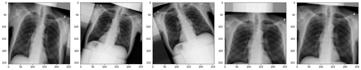
The images look a little strange, but that’s the idea! When our model sees something unusual in real-life, it will be better adapted to deal with it.
Now we have some data to work with, let’s start building our model.
MATLAB
Loading data to an array
Reading data from files and writing data to them are essential tasks in scientific computing, and something that we’d rather not spend a lot of time thinking about. Fortunately, MATLAB comes with a number of high-level tools to do these things efficiently, sparing us the grisly detail.
Before we get started, however, let’s create some directories to help organise this project.
Tip: Good Enough Practices for Scientific Computing
Good Enough Practices for Scientific Computing is a paper written by researchers involved with the Carpentries, which covers basic workflow skills for research computing. It recommends the following for project organization:
- Put each project in its own directory, which is named after the project.
- Put text documents associated with the project in the
docdirectory. - Put raw data and metadata in the
datadirectory, and files generated during clean-up and analysis in aresultsdirectory. - Put source code for the project in the
srcdirectory, and programs brought in from elsewhere or compiled locally in thebindirectory. - Name all files to reflect their content or function.
We already have a data directory in our
matlab-novice-inflammation project directory, so we only
need to create results and src directories for
this project. You can use your computer’s file browser to create this
directory.
A final step is to set the current folder in MATLAB to our project folder. Use the Current Folder window in the MATLAB GUI to browse to your project folder (the one now containing the ‘data’ and ‘results’ directories).
To verify the current directory in matlab we can run pwd
(print working directory). A second check we can do is to run the
ls (list) command in the Command Window to list the
contents of the working directory — we should get the following
output:
OUTPUT
data results srcWe are now set to load our data.
If we know what our data looks like (in this case, we have a matrix
stored as comma-separated values) and we’re unsure about what command we
want to use, we can search the documentation. Type
read matrix into the documentation toolbar. MATLAB suggests
using readmatrix. If we have a closer look at the
documentation, MATLAB also tells us, which inputs and output this
function has.
For the readmatrix function we need to provide a single
argument: the path to the file we want to read
data from. Since our data is in the ‘data’ folder, the path will begin
with “data/”, and will be followed by the name of the file:
This loads the data and assigns it to a variable, patient_data. This is a good example of when to use a semi-colon to suppress output — try re-running the command without the semi-colon to find out why. You should see a wall of numbers printed, which is the data from the file.
We can see in the workspace that the variable has 60 rows and 40
columns. If you can’t see the workspace, you can check this with
size, as we did before:
OUTPUT
ans =
    60 40
You might also recognise the icon in the workspace telling you that
the variable is of type double. If you don’t, you can use the
class function to find out what type of data lives inside
an array:
OUTPUT
ans =
    'double'
Again, this just means that you can store very small or very large numbers, called double precision floating-point numbers.
Initial exploration
We know that in our data each row represents a patient and each column a different day.
One patient at a time
We know how to access sections of our data, so lets look at a single patient first. If we want to look at a single patients’ data, then, we have to get all the columns for a given row, with:
OUTPUT
patient_5 =
  Columns 1 through 25
     0     1     1     3     3     1     3     5     2     4     4     7     6     5     3    10     8    10     6    17     9    14     9     7    13
  Columns 26 through 40
     9    12     6     7     7     9     6     3     2     2     4     2     0     1     1
Looking at these 40 numbers tells us very little, so we might want to look at the mean instead, for example.
OUTPUT
mean_p5 =
    5.5500
We can also compute other statistics, like the maximum, minimum and standard deviation.
OUTPUT
max_p5 =
    17
min_p5 =
     0
std_p5 =
    4.1072
All data points at once
Can you think of a way to get the mean of the whole data? What about
the max, min and std?
We already know that the colon operator as an index returns all the
elements, so patient_data(:) will return a vector with all
the data points. To compute the mean, we then use:
OUTPUT
global_mean =
    6.1487
This works for max, min and
std too:
MATLAB
>> global_max = max(patient_data(:))
>> global_min = min(patient_data(:))
>> global_std = std(patient_data(:))
OUTPUT
global_max =
    20
global_min =
     0
global_std =
    4.6148
Now that we have the global statistics, we can check how patient 5 compares with them:
MATLAB
>> mean_p5 > global_mean
>> max_p5 == global_max
>> min_p5 == global_min
>> std_p5 < global_std
ans =
logical
0
ans =
logical
0
ans =
logical
1
ans =
logical
1So we know that patient 5 did not suffer more inflamation than average, that it is not the patient who got the most inflamed, that he had the global minimum inflamation at some point (0), and that the std of his inflamation is not below the average.
Food for thought
How would you find the patient who got the highest inflamation?
Would you be happy to do it if you had 1000 patients?
One day at a time
We could also have looked not at a single patient, but at a single day. The approach would be very similar, but instead of selecting all the columns in a row, we want to select all the rows for a given column:
The result is now not a row of 40 elements, but a column with 60 items. However, matlab is smart enough to figure out what to do with enquieries just like the ones we did before.
MATLAB
>> mean_d9 = mean(day_9)
>> max_d9 = max(day_9)
>> min_d9 = min(day_9)
>> std_d9 = std(day_9)
OUTPUT
mean_d9 =
     5.2333
max_d9 =
     8
min_d9 =
     2
std_d9 =
    1.9430
We could now check how day 9 compares to the global values:
MATLAB
>> mean_d9 > global_mean
>> max_d9 == global_max
>> min_d9 == global_min
>> std_d9 < global_std
ans =
logical
0
ans =
logical
0
ans =
logical
0
ans =
logical
1So we know that day 9 was still relatively low inflamation, that it is not the day with the highest inflamation, that every patient was at least a bit inflamed at that moment, and that the std of his inflamation is below the average (so datapoints are closer to each other).
Food for thought
How would you find which days had an inflamation value above the global mean?
Would you be happy to do it if you had 1000 days worth of data?
Whole array analisis
The analisis we’ve done until now would be very tedious to repeat for each patient or day. Luckily, we’ve been telling you that matlab is used to thinking in terms of arrays. Surely then, it must be possible to get the mean of each patient or each day in one go. It is definitely tempting to simply call the mean on the array, so let’s try it:
We’ve supressed the output, but the workspace (or use of
size) tells us that the result is a 1x40 array. Matlab
assumed that we want column averages, and indeed that is something we
might want.
The other statistics behave in the same way, so we can more appropriately label our variables as:
MATLAB
>> per_day_mean = mean(patient_data);
>> per_day_max = max(patient_data);
>> per_day_min = min(patient_data);
>> per_day_std = std(patient_data);
You’ll notice that each of the above avriables is a 1x40
array.
Now that we have the information for each day in an array, we can take advantage of Matlab’s capacity to do array operations. For example, we can find out which days had an inflamation above the global average:
ans =
  1×40 logical array
  Columns 1 through 14
   0   0   0   0   0   0   0   0   0   0   0   0   1   1

  Columns 15 through 28
   1   1   1   1   1   1   1   1   1   1   1   1   1   1

  Columns 29 through 40
   1   1   0   0   0   0   0   0   0   0   0   0
We could count which day it is, but lets take a shortcut and use the find function:
ans =
  Columns 1 through 9
    13    14    15    16    17    18    19    20    21

  Columns 10 through 18
    22    23    24    25    26    27    28    29    30
So it seems that days 13 to 30 were the critical days.
But what if we want the analysis per patient, instead of per day?
Lets look at the documentation for mean, either through
the documentation browser or using the help command
OUTPUT
mean   Average or mean value.
    S = mean(X) is the mean value of the elements in X if X is a vector.
    For matrices, S is a row vector containing the mean value of each
    column.
    For N-D arrays, S is the mean value of the elements along the first
    array dimension whose size does not equal 1.

    mean(X,DIM) takes the mean along the dimension DIM of X.

    S = mean(...,TYPE) specifies the type in which the mean is performed,
    and the type of S. Available options are:

    'double'    -  S has class double for any input X
    'native'    -  S has the same class as X
    'default'   -  If X is floating point, that is double or single,
                   S has the same class as X. If X is not floating point,
                   S has class double.

    S = mean(...,NANFLAG) specifies how NaN (Not-A-Number) values are
    treated. The default is 'includenan':

    'includenan' - the mean of a vector containing NaN values is also NaN.
    'omitnan'    - the mean of a vector containing NaN values is the mean
                   of all its non-NaN elements. If all elements are NaN,
                   the result is NaN.

    Example:
        X = [1 2 3; 3 3 6; 4 6 8; 4 7 7]
        mean(X,1)
        mean(X,2)

    Class support for input X:
       float: double, single
       integer: uint8, int8, uint16, int16, uint32,
                int32, uint64, int64

    See also median, std, min, max, var, cov, mode.
The first paragraph explains why it worked for a single day or patient. The input we used was a vector, so it took the mean.
The second paragraph explains why we got per-day means when we used the whole data as input. Our array is 2D, and the first dimention is the rows, so it averaged the rows.
The third paragraph is the key to what we want to do now. A second
argument DIM can be used to specify the direction in which
to take the mean. If we want patient averages, we want the columns to be
averaged, that is, dimension 2.
As expected, the result is a 60x1 vector, with the mean
for each patient.
Unfortunately, max, min and
std do not behave quite in the same way. If you explore
their documentation, you’ll see that we need to add another argument, so
that the commands become:
MATLAB
>> per_patient_max = max(patient_data,[],2);
>> per_patient_min = min(patient_data,[],2);
>> per_patient_std = std(patient_data,[],2);
All of the above return a 60x1 vector.
Most inflamed patients
Can you find the patients that got the highest inflamation?
Using the power matlab has to compare arrays, we can check which
patients have a max equal to the global_max.
If we wrap this check in the find function, we get the row numbers:
ans =
     8
    29
    52
So the patients 8, 29 and 52 got the maximum inflamation levels.
We can gain some insight exploring the data like we have so far, but we all know that an image speaks more than a thousend numbers, so we’ll learn to make some plots.
Key Points
- “Data augmentation can help to avoid overfitting.”