Loading data
Last updated on 2025-02-28 | Edit this page
Estimated time: 40 minutes
Overview
Questions
- How can I load data to an array?
Objectives
- Read data from a csv to be able to work with it in matlab.
- Familiarize ourselves with our sample data.
Loading data to an array
Reading data from files and writing data to them are essential tasks in scientific computing, and something that we’d rather not spend a lot of time thinking about. Fortunately, MATLAB comes with a number of high-level tools to do these things efficiently, sparing us the grisly detail.
Before we get started, however, let’s make sure we have the directories to help organise this project.
Tip: Good Enough Practices for Scientific Computing
Good Enough Practices for Scientific Computing is a paper written by researchers involved with the Carpentries, which covers basic workflow skills for research computing. It recommends the following for project organization:
- Put each project in its own directory, which is named after the project.
- Put text documents associated with the project in the
docdirectory. - Put raw data and metadata in the
datadirectory, and files generated during clean-up and analysis in aresultsdirectory. - Put source code for the project in the
srcdirectory, and programs brought in from elsewhere or compiled locally in thebindirectory. - Name all files to reflect their content or function.
We already have a data, results and
src directories in our
matlab-novice-inflammation project directory, so we are
ready to continue.
A final step is to set the current folder in MATLAB to our project folder. Use the Current Folder window in the MATLAB GUI to browse to your project folder (the one now containing the ‘data’, ‘results’ and ‘src’ directories).
To verify the current directory in MATLAB we can run pwd
(print working directory).
OUTPUT
.../Desktop/matlab-novice-inflammationA second check we can do is to run the ls (list) command
in the Command Window to list the contents of the working directory — we
should get the following output:
OUTPUT
data results srcWe are now set to load our data. As a reminder, our data is structured like this:
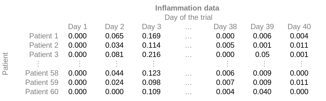
But it is stored without the headers, as comma-separated values. Each
line in the file corresponds to a row, and the value for each column is
separated from its neighbours by a comma. The first few rows of our
first file, data/base/inflammation-01.csv, look like
this:
0,0.065,0.169,0.271,0.332,0.359,0.354,0.333,0.304,0.268,0.234,0.204,0.179,0.141,0.133,0.115,0.083,0.076,0.065,0.065,0.047,0.04,0.041,0.028,0.02,0.028,0.012,0.02,0.011,0.015,0.009,0.01,0.01,0.007,0.007,0.001,0.008,-0,0.006,0.004
0,0.034,0.114,0.2,0.272,0.321,0.328,0.32,0.314,0.287,0.246,0.215,0.207,0.171,0.146,0.131,0.107,0.1,0.088,0.065,0.061,0.052,0.04,0.042,0.04,0.03,0.031,0.031,0.016,0.019,0.02,0.017,0.019,0.006,0.009,0.01,0.01,0.005,0.001,0.011
0,0.081,0.216,0.277,0.273,0.356,0.38,0.349,0.315,0.23,0.235,0.198,0.106,0.198,0.084,0.171,0.126,0.14,0.086,0.01,0.06,0.081,0.022,0.035,0.01,0.086,-0,0.102,0.032,0.07,0.017,0.136,0.022,-0,0.031,0.054,-0,-0,0.05,0.001
There is a very tempting button that says “Import Data” in the toolbar. If you click on it, you can find the file, and it will take you through a GUI wizard to upload the data. However, this is much more complicated than what we need, and it is not very helpful for loading multiple files (as we will in later episodes). Instead, lets try to do it on the command window.
We can search the documentation to try to learn how to read our
matrix of data. Type read matrix into the documentation
toolbar. MATLAB suggests using readmatrix. If we have a
closer look at the documentation, MATLAB also tells us which inputs and
output this function has.
For the readmatrix function we need to provide a single
argument: the path to the file we want to read
data from. Since our data is in the ‘data’ folder, the path will begin
with “data/”, we’ll also need to specify the subfolder (we will start by
using “base/”), and this will be followed by the name of the file:
This loads the data and assigns it to a variable, patient_data. This is a good example of when to use a semi-colon to suppress output — try re-running the command without the semi-colon to find out why. You should see a wall of numbers printed, which is the data from the file.
We can see in the workspace that the variable has 60 rows and 40
columns. If you can’t see the workspace, you can check this with
size, as we did before:
OUTPUT
ans =
    60 40
You might also recognise the icon in the workspace telling you that
the variable is of type double. If you don’t, you can use the
class function to find out what type of data lives inside
an array:
OUTPUT
ans =
    'double'
Again, this just means that you can store very small or very large numbers, called double precision floating-point numbers.
Initial exploration
We know that in our data each row represents a patient and each column a different day.
One patient at a time
We know how to access sections of our data, so lets look at a single patient first. If we want to look at a single patients’ data, then, we have to get all the columns for a given row, with:
OUTPUT
patient_5 =
  Columns 1 through 14
         0    0.0370    0.1330    0.2280    0.3060    0.3410    0.3410    0.3480    0.3160    0.2750    0.2540    0.2250    0.1870    0.1630
  Columns 15 through 28
    0.1440    0.1190    0.1070    0.0880    0.0720    0.0600    0.0510    0.0510    0.0390    0.0330    0.0240    0.0280    0.0170    0.0200
  Columns 29 through 40
    0.0160    0.0200    0.0190    0.0180    0.0070    0.0160    0.0220    0.0180    0.0150    0.0050    0.0100    0.0100
Looking at these 40 numbers tells us very little, so we might want to look at the mean instead, for example.
OUTPUT
mean_p5 =
    0.1046
We can also compute other statistics, like the maximum, minimum and standard deviation.
OUTPUT
max_p5 =
    0.3480
min_p5 =
     0
std_p5 =
0.1142All data points at once
Can you think of a way to get the mean of the whole data? What about
the max?
We already know that the colon operator as an index returns all the
elements, so patient_data(:) will return a vector with all
the data points. To compute the mean, we then use:
OUTPUT
global_mean =
    0.1053
This works for max too:
OUTPUT
global_max =
    0.4530
Now that we have the global statistics, we can check how patient 5 compares with them:
ans =
  logical
   0
ans =
  logical
   0
So we know that patient 5 did not suffer more inflammation than average, and that they are not the patient who got the most inflamed.
One day at a time
We could also have looked not at a single patient, but at a single day. The approach would be very similar, but instead of selecting all the columns in a row, we want to select all the rows for a given column:
The result is now not a row of 40 elements, but a column with 60 items. However, MATLAB is smart enough to figure out what to do with enquiries just like the ones we did before.
OUTPUT
mean_d9 =
    0.3116
max_d9 =
    0.3780
Whole array analysis
The analysis we’ve done until now would be very tedious to repeat for each patient or day. Luckily, we’ve learnt that MATLAB is used to thinking in terms of arrays. Surely it must be possible to get the mean of each patient or each day in one go. It is definitely tempting to simply call the mean on the array, so let’s try it:
We’ve suppressed the output, but the workspace (or use of
size) tells us that the result is a 1x40 array. Matlab
assumed that we want column averages, and indeed that is something we
might want.
The other statistics behave in the same way, so we can more appropriately label our variables as:
You’ll notice that each of the above variables is a 1×40
array.
Now that we have the information for each day in an array, we can take advantage of Matlab’s capacity to do array operations. For example, we can find out which days had an inflammation above the global average:
ans =
  1×40 logical array
  Columns 1 through 20
   0   0   1   1   1   1   1   1   1   1   1   1   1   1   1   1   1   0   0   0
  Columns 21 through 40
   0   0   0   0   0   0   0   0   0   0   0   0   0   0   0   0   0   0   0   0
We could count which day it is, but lets take a shortcut and use the find function:
ans =
     3     4     5     6     7     8     9    10    11    12    13    14    15    16    17
So it seems that days 3 to 17 were the critical days.
Per patient analysis
We have seen that mean and max can compute
the per day statistics if we called them on the whole array.
But how can we get the per patient statistics?
Lets look at the documentation for mean, either through
the documentation browser or using the help command
OUTPUT
mean   Average or mean value.
    S = mean(X) is the mean value of the elements in X if X is a vector.
    For matrices, S is a row vector containing the mean value of each
    column.
    For N-D arrays, S is the mean value of the elements along the first
    array dimension whose size does not equal 1.

    mean(X,DIM) takes the mean along the dimension DIM of X.

    S = mean(...,TYPE) specifies the type in which the mean is performed,
    and the type of S. Available options are:

    'double'    -  S has class double for any input X
    'native'    -  S has the same class as X
    'default'   -  If X is floating point, that is double or single,
                   S has the same class as X. If X is not floating point,
                   S has class double.

    S = mean(...,NANFLAG) specifies how NaN (Not-A-Number) values are
    treated. The default is 'includenan':

    'includenan' - the mean of a vector containing NaN values is also NaN.
    'omitnan'    - the mean of a vector containing NaN values is the mean
                   of all its non-NaN elements. If all elements are NaN,
                   the result is NaN.

    Example:
        X = [1 2 3; 3 3 6; 4 6 8; 4 7 7]
        mean(X,1)
        mean(X,2)

    Class support for input X:
       float: double, single
       integer: uint8, int8, uint16, int16, uint32,
                int32, uint64, int64

    See also median, std, min, max, var, cov, mode.
The first paragraph explains why it worked for a single day or patient. The input we used was a vector, so it took the mean.
The second paragraph explains why we got per-day means when we used the whole data as input. Our array is 2D, and the first dimension is the rows, so it averaged the rows.
The third paragraph is the key to what we want to do now. A second
argument DIM can be used to specify the direction in which
to take the mean. If we want patient averages, we want the columns to be
averaged, that is, dimension 2.
As expected, the result is a 60×1 vector, with the mean
for each patient.
Unfortunately, max does not behave quite in the same
way. If you explore its documentation, you’ll see that we need to add
another argument, so that the command becomes:
We can gain some insight exploring the data like we have so far, but we all know that an image speaks more than a thousand numbers, so we’ll learn to make some plots.
- Use
readmatrixto read tabular CSV data into a program. - Use
mean,min,max, andstdon vectors to get the mean, minimum, maximum and standard deviation. - Use
mean(array,DIM)to specify the dimension of your array in which to compute the mean. - For
min,max, andstd, the arguments need to be(array,[],DIM)instead.