All in One View
Content from Working With Variables
Last updated on 2025-02-28 | Edit this page
Estimated time: 50 minutes
Overview
Questions
- How can I store values and do simple calculations with them?
- Which type of operations can I do?
Objectives
- Navigate among important sections of the MATLAB environment.
- Assign values to variables.
- Identify what type of data is stored in a variable.
- Creating simple arrays.
- Be able to explore the values of saved variables.
- Learn how to delete variables and keep things tidy.
Introduction to the MATLAB GUI
Before we can start programming, we need to know a little about the MATLAB interface. Using the default setup, the MATLAB desktop contains several important sections:
- In the Command Window we can execute commands.
Commands are typed after the prompt
>>and are executed immediately after pressing Enter. - Alternatively, we can open the Editor, write our code and run it all at once. The advantage of this is that we can save our code and run it again in the same way at a later stage.
- The Workspace contains all the variables which we have loaded into memory.
- The Current Folder window shows files in the current directory. We can change the current folder using this window.
-
Search Documentation on the top right of your
screen lets you search for functions. Suggestions for functions that
will do what you want to do will pop up. Clicking on them will open the
documentation. Another way to access the documentation is via the
helpcommand — we will return to this later.
Working with variables
In this lesson we will learn how to manipulate the inflammation dataset with MATLAB. But before we discuss how to deal with many data points, we will demonstrate how to store a single value on the computer.
We can create a new variable by
assigning a value to it using =
OUTPUT
x =
    55
Notice that MATLAB responded by printing an output confirming that the variable has the desired value, and also that the variable appeared in the workspace.
A variable is just a name for a piece of data or value.
Variable names must begin with a letter, and are case sensitive. They
can also contain numbers or underscores. Examples of valid variable
names are weight, size3,
patient_name or alive_on_day_3.
The reason we work with variables is so that we can reuse them, or save them for later use. We can also do operations with these variables. For example, we can do a simple sum:
OUTPUT
y =
    10
ans =
    65
Note that the answer was saved in a new variable called
ans. This variable is temporary, and will be overwritten
with any new operation we do. For example, if we now substract y from x
we get:
OUTPUT
ans =
    45
The result of the sum is now gone forever. We can assign the result of an operation to a new variable, for example:
OUTPUT
z =
    550
This created a new variable z. If you look at the
workspace, you can see that the value of z is 550.
We can even use a variable in an operation, and save the value in the same variable. For example:
OUTPUT
y =
    2
Here you can see that the expression to the right of the
= sign is evaluated first, and the result is then
assigned to the variable specified to the left of the =
sign.
We can use multiple variables in a single operation, for example:
OUTPUT
z =
    817
where we used the caret symbol ^ to take the third power
of y.
Logical operations
In programming, there is another type of operation that becomes very important: comparison. We can compare two numbers (or variables) to see which one is smaller, for example
OUTPUT
mass =
    20
age =
    2.5000
frac =
     8

c1 =
  logical
   1
Something interesting just happened with the variable c1. If I ask
you whether frac (8) is smaller than 10, you would say “yes”. Matlab
answered with a logical 1. If I ask you whether frac is
greater than 10, you would say “no”. Matlab answers with a
logical 0.
OUTPUT
c2 =
  logical
   0
There are only two options (yes or no, true or false, 0 or 1), and so it is “cheaper” for the computer to save space only for those two options.
The “type” of this data is not the same as the “type” of data that represents a number. It comes from a logical comparison, and so MATLAB identifies it as such.
You can also see that in the workspace these variables have a tick next to them, instead of the squares we had seen. There are actually other symbols that appear there, relating to the different types of information we can save in variables (unfold the info below if you want to know more).
Data types
We mentioned above that we can get other symbols in the workspace which relate to the types of information we can save.
We know we can save numbers, and logical values, but we can also save letters or strings, for example. Numbers are by default saved as type double, which means they can store very big or very small numbers. Letters are type ‘char’, and words or sentences are “strings”. Logical values (or booleans) are values that mean true or false, and are represented with zero or one. They are usually the result of comparing things.
OUTPUT
weight =
   64.5000
size3 =
    'L'
patient_name =
    "Jane Doe"
alive_on_day_3 =
  logical
   1
Notice the single tick for character variables, in contrast with the double quote for strings.
If you look at the workspace, you’ll notice that the icon next to each variable is different, and if you hover over it, it will tell you the type of variable it is.
You can also check the “class” of the variable with the
class function:
OUTPUT
ans =
    'string'
We can also check if two variables (or even operations) are the same
OUTPUT
c3 =
  logical
   1
We can also combine comparisons. For example, we can check whether frac is smaller than 10 and the age is greater than 2.5
OUTPUT
c4 =
  logical
   0
In this case, both conditions need to be met for the result to be “yes” (1).
If we want a “yes” as long as at least one of the conditions are met, we would ask if frac is smaller than 10 or the age is greater than 2.5
OUTPUT
c5 =
  logical
   1
It is quite common to want to include the limits in a comparison. For example, we might want to know if a number is greater or equal to another. We could construct this with two comparisons, one for greater and one for equal:
OUTPUT
c6 =
  logical
   0
This is so common, however, that MATLAB has the special combinations
saved for this: >= and <=.
Finally, we often asks questions or state things in negative. “We did not start late today.”, “I was not going faster than the speed limit officer!”, and “I didn’t shoot no deputy” are just some examples.
Naturally, we may want to do so in programming too. In MATLAB the
negative is represented with ~. For example, we can check
if the speed is indeed not faster than the limit with:
OUTPUT
ans =
  logical
   1
which MATLAB reads as “not speed greater than 70”.
Conditionals
Can you express these questions in MATLAB code?
Note: make sure that x=55 and
y=2 are defined before you start!
- Is 1 + 2 + 3 + 4 smaller than 10?
- Is 1 + 2 + 3 + 4 not smaller than 10?
- Is 5 to the power of 3 equal to 125?
- Is 5 to the power of 3 different from 125?
- Is x + y smaller than x/y?
- Is x + y not smaller than x/y?
- Is x + y greater or equal to x/y?
- Is x + y not greater or equal to x/y?
MATLAB
>> 1 + 2 + 3 + 4 < 10     # false
>> ~(1 + 2 + 3 + 4 < 10)  # true
>> 5^3 == 125             # true
>> ~(5^3 == 125)          # false - Can also be: 5^3 ~= 125
>> x+y < x/y              # false
>> ~(x+y < x/y)           # true
>> x+y >= x/y             # true - same as the previous one!
>> ~(x+y >= x/y)          # false - same as x+y < x/y
Asking if two things are different is so common, that MATLAB has a
special symbol for it: ~=. The fourth question,then, we
could have asked instead as 5^3 ~= 125. Unfortunately,
there is no special symbol for negating the >,
<, >=, and <=
comparisons. As we have seen, however, if we are clever with which one
we use, the come for free!
Arrays
You may notice that all of the variable types start with a
1x1. This is because MATLAB thinks in terms of
groups of variables called arrays, or matrices.
We can create an array using square brackets and separating each value with a comma:
OUTPUT
A =
     1     2     3
If you now hover over the data type icon, you’ll find that it shows
1x3. This means that the array A has 1
row and 3
columns.
We can create matrices using semi-colons to separate rows:
OUTPUT
B =
     1     2
     3     4
     5     6
You’ll notice that B has three rows and two columns, which explains
the 3x2 we get from the workspace.
We can also create arrays of other types of data. For example, we could create an array of names:
OUTPUT
Names =
  1×4 string array
    "John"    "Abigail"    "Bertrand"    "Lucile"
We can use logical values too:
OUTPUT
C =
  4×1 logical array
   1
   0
   0
   1
Something to bear in mind, however, is that all values in an array must be of the same type.
We mentioned before that MATLAB is actually more used to working with arrays than individual variables. Well, if it is so used to working with arrays, can we do operations with them?
The answer is yes! In fact, this is what makes MATLAB a particularly interesting programming language.
We can, for example, check the whole matrix B and look for values greater than, say, 3.
OUTPUT
ans =
  3×2 logical array
   0   0
   0   1
   1   1
MATLAB then compared each element of B and asked “is this element greater than 3?”. The result is another array, of the same size and dimensions as B, with the answers.
We can also do sums, multiplications, and pretty much anything we want with an array, but we need to be careful with what we do.
Despite this being so interesting and increadibly powerful, this course will focus more on basic programming concepts, and so we won’t use this feature very much. However, it is very important that you keep it in mind, and that you do ask questions about it during the break if you are interested.
Suppressing the output
In general, the output can be a bit redundant (or even annoying!), and it can make the code slower, so it is considered good form to suppress it. To suppress it, we add a semi-colon at the end of the line:
At first glance nothing appears to have happened, but the workspace shows the new value was assigned.
Printing a variable’s value
If we really want to print the variable, then we can simply type its name and hit Enter,
OUTPUT
patient_name =

    "Jane Doe"
or using the disp
function.
Functions are pre-defined algorithms (chunks of code), that can be used multiple times. They usually take some “inputs” inside brackets, and either have an effect on something or output something.
The disp function, in particular, takes just one input – the variable that you want to print – and what it does is to print the variable in a nice way. For the variable patient_name, we would use it like this:
OUTPUT
Jane DoeNote how the output is a bit different from what we got when we just typed the variable name. There is less indentation and less empty lines.
Keeping things tidy
We have declared a few variables now, and we might not be using all
of them. If we want to delete a variable we can do so by typing
clear and the name of the variable, e.g.:
You might be able to see it disappear from the workspace. If you now try to use alive_on_day_3, MATLAB will give an error.
We can also delete all of our variables with the
command clear, without any variable names following it. Be
careful though, there’s no way back!
Another thing you might want to clear every once in a while is the
output pane. To do that, we use the command clc.
Again, be careful usig this command, there is no way back!
- Variables store data for future use. Their names must start with a letter, and can have underscores and numbers.
- We can add, substract, multiply, divide and potentiate numbers.
- We can also compare variables with
<,>,==,>=,<=,~=, and use~to negate the result. - Combine logical operations with
&&(and) and||(or). - MATLAB stores data in arrays. The data in an array has to be of the same type.
- You can supress output with
;, and print a variable withdisp. - Use
clearto delete variables, andclcto clear the console.
Content from Arrays
Last updated on 2024-03-22 | Edit this page
Estimated time: 40 minutes
Overview
Questions
- How can I access the information in an array?
Objectives
- Learn how to create multidimensional arrays
- Select individual values and subsections of an array.
Initializing an Array
We just talked about how MATLAB thinks in arrays, and
declared some very simple arrays using square brackets. In some cases,
we will want to create space to save data, but not save anything just
yet. One way of doing so is with zeros. The function zeros
takes the dimensions of our array as arguments, and populates it with
zeros. For example,
OUTPUT
Z =
     0     0     0     0     0
     0     0     0     0     0
     0     0     0     0     0
creates a matrix of 3 rows and 5 columns, filled with zeros. If we had only passed one dimension, MATLAB assumes you want a square matrix, so
OUTPUT
Z =
     0     0     0
     0     0     0
     0     0     0
yields a 3×3 array. If we want a single row and 5 columns, we need to
remember that MATLAB reads rows×columns,
so
OUTPUT
Z =
     0     0     0     0     0
This way zeros function works is shared with many other
functions that create arrays.
For example, the ones
function is nearly identical, but the arrays are filled with ones,
and the rand
function assigns uniformly distributed random numbers between zero
and 1 to each space in the array.
Note: This is when supressing the output becomes
more important. You can more comfortably explore the variables
R and O by double clicking them in the
workspace.
The ones function can actually help us initialize a
matrix to any value, because we can multiply a matrix by a constant and
it will multiply each element. So for example,
Produces a 3×6 matrix full of fives.
The magic
function works in a similar way, but you can only declare square
matrices with it. The magic thing about them is that the sum of the
elements on each row or column is the same number.
OUTPUT
M =
    16     2     3    13
     5    11    10     8
     9     7     6    12
     4    14    15     1
In this case, each row or column adds up to 34. But how could I tell in a bigger matrix? How can I select some of the elements of the array and sum them, for example?
Array indexing
Array indexing, is the method by which we can select one or more different elements of an array. A solid understanding of array indexing will be essential to working with arrays. Lets start with selecting one element.
First, we will create an 8×8 “magic” matrix:
OUTPUT
ans =

   64    2    3   61   60    6    7   57
    9   55   54   12   13   51   50   16
   17   47   46   20   21   43   42   24
   40   26   27   37   36   30   31   33
   32   34   35   29   28   38   39   25
   41   23   22   44   45   19   18   48
   49   15   14   52   53   11   10   56
    8   58   59    5    4   62   63    1
We want to access a single value from the matrix:

To do that, we must provide its index in
parentheses. In a 2D array, this means the row and column of the element
separated by a comma, that is, as (row, column). This index
goes after the name of our array. In our case, this is:
OUTPUT
ans = 38So the index (5, 6) selects the element on the fifth row
and sixth column of M.
Note: Matlab starts counting indices at 1, not 0! Many other programming languages start counting indices at 0, so be careful!.
An index like the one we used selects a single element of an array, but we can also select a group of elements if instead of a number we give arrays of indices. For example, if we want to select this submatrix:

we want rows 4, 5 and 6, and columns 5, 6 and 7, that is, the arrays
[4,5,6] for rows, and [5,6,7] for columns:
OUTPUT
ans =
   36   30   31
   28   38   39
45 19 18The : operator
In matlab, the symbol : (colon)
is used to specify a range. The range is specified as
start:end. For example, if we type 1:6 it
generates an array of consecutive numbers from 1 to 6:
OUTPUT
ans =
   1     2     3     4     5     6
We can also specify an increment other than one. To specify
the increment, we write the range as start:increment:end.
For example, if we type 1:3:15 it generates an array
starting with 1, then 1+3, then 1+2*3, and so on, until it reaches 15
(or as close as it can get to 15 without going past it):
OUTPUT
ans =
   1     4     7    10    13
The array stopped at 13 because 13+3=16, which is over 15.
The rows and columns we just selected could have been specified as
ranges. So if we want the rows from 4 to 6 and columns from 5 to 7, we
can specify the ranges as 4:6 and 5:7. On top
of being a much quicker and neater way to get the rows and columns,
MATLAB knows that the range will produce an array, so we do not even
need the square brackets anymore. So the command above becomes:
OUTPUT
ans =
   36   30   31
   28   38   39
45 19 18Checkerboard
Select the elements highlighted on the image:

Selecting whole rows or columns
If we want a whole row, for example:

we could in principle pick the 5th row and for the columns use the
range 1:8.
OUTPUT
ans =
   32   34   35   29   28   38   39   25
However, we need to know that there are 8 columns, which is not very robust.
The key-word end
When indexing the elements of an array, the key word end
can be used to get the last index available.
For example, M(2, end) returns the last element of the
second row:
OUTPUT
ans =
   16
We can also use it in combination with the : operator.
For example, M(5:end, 3) returns the elements of column 3
from row 5 until the end:
OUTPUT
ans =
   35
   22
   14
   59
We can then use the keyword end instead of the 8 to get
the whole row with 1:end.
OUTPUT
ans =
   32   34   35   29   28   38   39   25
This is much better, now this works for any size of matrix, and we don’t need to know the size.
As you can see, the : operator is quite important when
accessing arrays!
We can use it to select multiple rows,

OUTPUT
ans =
   64    2    3   61   60    6    7   57
    9   55   54   12   13   51   50   16
   17   47   46   20   21   43   42   24
   40   26   27   37   36   30   31   33
or multiple columns:

OUTPUT
ans =
    6    7   57
   51   50   16
   43   42   24
   30   31   33
   38   39   25
   19   18   48
   11   10   56
   62   63    1
or even the whole matrix. Try for example:
and you’ll see that it returns all the elements of M. The result,
however, is a column vector, not a matrix. We can make sure that the
result of M(:) has 8x8=64 elements by using the function size,
which returns the dimensions of the array given as an input:
OUTPUT
ans =
   64    1
So it has 64 rows and 1 column. Effectively, then, M(:)
‘flattens’ the array into a column vector. The order of the elements in
the resulting vector comes from appending each column of the original
array in turn. This is the result of something called linear
indexing, which is a way of accessing elements of an array by a
single index.
Master indexing
Select the elements highlighted on the image without using the
numbers 5 or 8, and using end only once:

Slicing character arrays
A subsection of an array is called a slice. We can take slices of character arrays as well:
MATLAB
>> element = 'oxygen';
>> disp("first three characters: " + element(1:3))
>> disp("last three characters: " + element(4:6))
OUTPUT
first three characters: oxy
last three characters: gen
And we can use all the tricks we have learned to select the data we want. For example, to select every other character we can use the colon operator with an increment of 2:
OUTPUT
ans =
    'oye'
We can also use the colon operator to access all the elements of the
array, but you’ll notice that the only difference between evaluating
element and element(:) is that the former is a
row vector, and the latter a column vector.
- Some functions to initialize matrices include
zeros,ones, andrand. They all produce a square matrix if only one argument is given, but you can specify the dimensions you want separated by a comma, as inzeros(rows,columns). - To select data points we use round brackets and provide the row and
column indices of the elements we want. They can be just numbers or
arrays of numbers, e.g.
M(5,[3,4,5]). - Use the colon operator
:to generate ordered arrays asstart:endorstart:increment:end. - Use the keyword
endto obtain the index of the final element. - The colon operator by itself
:selects all the elements.
Content from Loading data
Last updated on 2025-02-28 | Edit this page
Estimated time: 40 minutes
Overview
Questions
- How can I load data to an array?
Objectives
- Read data from a csv to be able to work with it in matlab.
- Familiarize ourselves with our sample data.
Loading data to an array
Reading data from files and writing data to them are essential tasks in scientific computing, and something that we’d rather not spend a lot of time thinking about. Fortunately, MATLAB comes with a number of high-level tools to do these things efficiently, sparing us the grisly detail.
Before we get started, however, let’s make sure we have the directories to help organise this project.
Tip: Good Enough Practices for Scientific Computing
Good Enough Practices for Scientific Computing is a paper written by researchers involved with the Carpentries, which covers basic workflow skills for research computing. It recommends the following for project organization:
- Put each project in its own directory, which is named after the project.
- Put text documents associated with the project in the
docdirectory. - Put raw data and metadata in the
datadirectory, and files generated during clean-up and analysis in aresultsdirectory. - Put source code for the project in the
srcdirectory, and programs brought in from elsewhere or compiled locally in thebindirectory. - Name all files to reflect their content or function.
We already have a data, results and
src directories in our
matlab-novice-inflammation project directory, so we are
ready to continue.
A final step is to set the current folder in MATLAB to our project folder. Use the Current Folder window in the MATLAB GUI to browse to your project folder (the one now containing the ‘data’, ‘results’ and ‘src’ directories).
To verify the current directory in MATLAB we can run pwd
(print working directory).
OUTPUT
.../Desktop/matlab-novice-inflammationA second check we can do is to run the ls (list) command
in the Command Window to list the contents of the working directory — we
should get the following output:
OUTPUT
data results srcWe are now set to load our data. As a reminder, our data is structured like this:
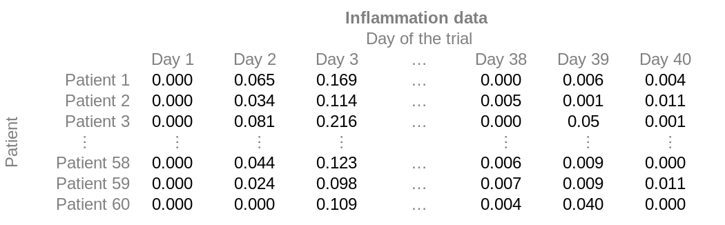
But it is stored without the headers, as comma-separated values. Each
line in the file corresponds to a row, and the value for each column is
separated from its neighbours by a comma. The first few rows of our
first file, data/base/inflammation-01.csv, look like
this:
0,0.065,0.169,0.271,0.332,0.359,0.354,0.333,0.304,0.268,0.234,0.204,0.179,0.141,0.133,0.115,0.083,0.076,0.065,0.065,0.047,0.04,0.041,0.028,0.02,0.028,0.012,0.02,0.011,0.015,0.009,0.01,0.01,0.007,0.007,0.001,0.008,-0,0.006,0.004
0,0.034,0.114,0.2,0.272,0.321,0.328,0.32,0.314,0.287,0.246,0.215,0.207,0.171,0.146,0.131,0.107,0.1,0.088,0.065,0.061,0.052,0.04,0.042,0.04,0.03,0.031,0.031,0.016,0.019,0.02,0.017,0.019,0.006,0.009,0.01,0.01,0.005,0.001,0.011
0,0.081,0.216,0.277,0.273,0.356,0.38,0.349,0.315,0.23,0.235,0.198,0.106,0.198,0.084,0.171,0.126,0.14,0.086,0.01,0.06,0.081,0.022,0.035,0.01,0.086,-0,0.102,0.032,0.07,0.017,0.136,0.022,-0,0.031,0.054,-0,-0,0.05,0.001
There is a very tempting button that says “Import Data” in the toolbar. If you click on it, you can find the file, and it will take you through a GUI wizard to upload the data. However, this is much more complicated than what we need, and it is not very helpful for loading multiple files (as we will in later episodes). Instead, lets try to do it on the command window.
We can search the documentation to try to learn how to read our
matrix of data. Type read matrix into the documentation
toolbar. MATLAB suggests using readmatrix. If we have a
closer look at the documentation, MATLAB also tells us which inputs and
output this function has.
For the readmatrix function we need to provide a single
argument: the path to the file we want to read
data from. Since our data is in the ‘data’ folder, the path will begin
with “data/”, we’ll also need to specify the subfolder (we will start by
using “base/”), and this will be followed by the name of the file:
This loads the data and assigns it to a variable, patient_data. This is a good example of when to use a semi-colon to suppress output — try re-running the command without the semi-colon to find out why. You should see a wall of numbers printed, which is the data from the file.
We can see in the workspace that the variable has 60 rows and 40
columns. If you can’t see the workspace, you can check this with
size, as we did before:
OUTPUT
ans =
    60 40
You might also recognise the icon in the workspace telling you that
the variable is of type double. If you don’t, you can use the
class function to find out what type of data lives inside
an array:
OUTPUT
ans =
    'double'
Again, this just means that you can store very small or very large numbers, called double precision floating-point numbers.
Initial exploration
We know that in our data each row represents a patient and each column a different day.
One patient at a time
We know how to access sections of our data, so lets look at a single patient first. If we want to look at a single patients’ data, then, we have to get all the columns for a given row, with:
OUTPUT
patient_5 =
  Columns 1 through 14
         0    0.0370    0.1330    0.2280    0.3060    0.3410    0.3410    0.3480    0.3160    0.2750    0.2540    0.2250    0.1870    0.1630
  Columns 15 through 28
    0.1440    0.1190    0.1070    0.0880    0.0720    0.0600    0.0510    0.0510    0.0390    0.0330    0.0240    0.0280    0.0170    0.0200
  Columns 29 through 40
    0.0160    0.0200    0.0190    0.0180    0.0070    0.0160    0.0220    0.0180    0.0150    0.0050    0.0100    0.0100
Looking at these 40 numbers tells us very little, so we might want to look at the mean instead, for example.
OUTPUT
mean_p5 =
    0.1046
We can also compute other statistics, like the maximum, minimum and standard deviation.
OUTPUT
max_p5 =
    0.3480
min_p5 =
     0
std_p5 =
0.1142All data points at once
Can you think of a way to get the mean of the whole data? What about
the max?
We already know that the colon operator as an index returns all the
elements, so patient_data(:) will return a vector with all
the data points. To compute the mean, we then use:
OUTPUT
global_mean =
    0.1053
This works for max too:
OUTPUT
global_max =
    0.4530
Now that we have the global statistics, we can check how patient 5 compares with them:
ans =
  logical
   0
ans =
  logical
   0
So we know that patient 5 did not suffer more inflammation than average, and that they are not the patient who got the most inflamed.
One day at a time
We could also have looked not at a single patient, but at a single day. The approach would be very similar, but instead of selecting all the columns in a row, we want to select all the rows for a given column:
The result is now not a row of 40 elements, but a column with 60 items. However, MATLAB is smart enough to figure out what to do with enquiries just like the ones we did before.
OUTPUT
mean_d9 =
    0.3116
max_d9 =
    0.3780
Whole array analysis
The analysis we’ve done until now would be very tedious to repeat for each patient or day. Luckily, we’ve learnt that MATLAB is used to thinking in terms of arrays. Surely it must be possible to get the mean of each patient or each day in one go. It is definitely tempting to simply call the mean on the array, so let’s try it:
We’ve suppressed the output, but the workspace (or use of
size) tells us that the result is a 1x40 array. Matlab
assumed that we want column averages, and indeed that is something we
might want.
The other statistics behave in the same way, so we can more appropriately label our variables as:
You’ll notice that each of the above variables is a 1×40
array.
Now that we have the information for each day in an array, we can take advantage of Matlab’s capacity to do array operations. For example, we can find out which days had an inflammation above the global average:
ans =
1×40 logical array
Columns 1 through 20
0 0 1 1 1 1 1 1 1 1 1 1 1 1 1 1 1 0 0 0
Columns 21 through 40
0 0 0 0 0 0 0 0 0 0 0 0 0 0 0 0 0 0 0 0We could count which day it is, but lets take a shortcut and use the find function:
ans =
3 4 5 6 7 8 9 10 11 12 13 14 15 16 17So it seems that days 3 to 17 were the critical days.
Per patient analysis
We have seen that mean and max can compute
the per day statistics if we called them on the whole array.
But how can we get the per patient statistics?
Lets look at the documentation for mean, either through
the documentation browser or using the help command
OUTPUT
mean Average or mean value.
S = mean(X) is the mean value of the elements in X if X is a vector.
For matrices, S is a row vector containing the mean value of each
column.
For N-D arrays, S is the mean value of the elements along the first
array dimension whose size does not equal 1.
mean(X,DIM) takes the mean along the dimension DIM of X.
S = mean(...,TYPE) specifies the type in which the mean is performed,
and the type of S. Available options are:
'double' - S has class double for any input X
'native' - S has the same class as X
'default' - If X is floating point, that is double or single,
S has the same class as X. If X is not floating point,
S has class double.
S = mean(...,NANFLAG) specifies how NaN (Not-A-Number) values are
treated. The default is 'includenan':
'includenan' - the mean of a vector containing NaN values is also NaN.
'omitnan' - the mean of a vector containing NaN values is the mean
of all its non-NaN elements. If all elements are NaN,
the result is NaN.
Example:
X = [1 2 3; 3 3 6; 4 6 8; 4 7 7]
mean(X,1)
mean(X,2)
Class support for input X:
float: double, single
integer: uint8, int8, uint16, int16, uint32,
int32, uint64, int64
See also median, std, min, max, var, cov, mode.The first paragraph explains why it worked for a single day or patient. The input we used was a vector, so it took the mean.
The second paragraph explains why we got per-day means when we used the whole data as input. Our array is 2D, and the first dimension is the rows, so it averaged the rows.
The third paragraph is the key to what we want to do now. A second
argument DIM can be used to specify the direction in which
to take the mean. If we want patient averages, we want the columns to be
averaged, that is, dimension 2.
As expected, the result is a 60×1 vector, with the mean
for each patient.
Unfortunately, max does not behave quite in the same
way. If you explore its documentation, you’ll see that we need to add
another argument, so that the command becomes:
We can gain some insight exploring the data like we have so far, but we all know that an image speaks more than a thousand numbers, so we’ll learn to make some plots.
- Use
readmatrixto read tabular CSV data into a program. - Use
mean,min,max, andstdon vectors to get the mean, minimum, maximum and standard deviation. - Use
mean(array,DIM)to specify the dimension of your array in which to compute the mean. - For
min,max, andstd, the arguments need to be(array,[],DIM)instead.
Content from Plotting data
Last updated on 2025-02-28 | Edit this page
Estimated time: 60 minutes
Overview
Questions
- How can I visualize my data?
Objectives
- Display simple graphs with appropriate titles and labels.
- Get familiar with the
plotfunction. - Learn how to plot multiple lines at the same time.
- Learn how to show images side by side.
- Get familiar with the
heatmapandimagescfunctions.
Plotting
The mathematician Richard Hamming once said, “The purpose of computing is insight, not numbers,” and the best way to develop insight is often to visualise data. Visualisation deserves an entire lecture (or course) of its own, but we can explore a few features of MATLAB here.
We will be using the data that we have loaded from
inflammation-01.csv and the per_day_mean and
per_day_max variables. If you haven’t done so, you can load
the data with:
MATLAB
>> patient_data = readmatrix("data/base/inflammation-01.csv");
>> per_day_mean = mean(patient_data);
>> per_day_max = max(patient_data);
>> patient_5 = patient_data(5,:);We will start by exploring the function plot. The most
common usage is to provide two vectors, like plot(X,Y).
Lets start by plotting the average inflammation across patients over
time. For the Y vector we can provide
per_day_mean, and for the X vector we want to
use the number of the day in the trial, which we can generate as a range
with:
Then our plot can be generated with:
Note: If we only provide a vector as an argument it
plots a data-point for each value on the y axis, and it uses the index
of each element as the x axis. For our patient data the indices coincide
with the day of the study, so plot(per_day_mean) generates
the same plot. In most cases, however, using the indices on the x axis
is not desirable.
Note: We do not even need to have the vector saved
as a variable. We would obtain the same plot with the command
plot(1:40, mean(patient_data, 1)), or
plot(mean(patient_data, 1)).
As it is, the image is not very informative. We need to give the
figure a title and label the axes using xlabel
and ylabel, so that other people can understand what it
shows (including us, if we return to this plot 6 months from now).

That’s much better! Now the plot actually communicates something. As we expected, this figure tells us way more than the numbers we had seen in the previous section.
Let’s have a look at the maximum inflammation per day across all patients.

Oh no! all our labels are gone!, we need to add them back, but this is going to be tedious…
Scripts
We often have to repeat a series of commands to achieve what we want, like with these plots. To be able to reuse our commands with more ease, we use scripts.
A more in depth exploration of scripts will be covered on the next
episode. For now, we’ll just start by clicking
new->script, using ctrl+N, or typing
edit on the command window.
Any of the above should open a new “Editor” window. Save the file
inside the src folder, as single_plot.m.
Alternatively, if you run
it creates the file with the correct path and name for you.
Note: Make sure to add the src folder
to your path, so that MATLAB knows where to find the script. To do that,
right click on the src directory, go to “Add to Path” and
to “Selected Folders”. Alternatively, run:
Try copying and pasting the plot commands for the max inflammation on the script and clicking on the “Run” button!
We can actually also include the data loading and the calculation of the mean and max in the script, so it will look like:
MATLAB
% *Script* to load data and plot inflammation values

% Load the data
patient_data = readmatrix("data/base/inflammation-01.csv");
per_day_mean = mean(patient_data);
per_day_max = max(patient_data);
patient_5 = patient_data(5,:);
day_of_trial = 1:40;

% Plot
plot(day_of_trial, per_day_mean)
title("Mean inflammation per day")
xlabel("Day of trial")
ylabel("Inflammation")
Because we now have a script, it should be much easier to change the plot to plot the max values:
MATLAB
% *Script* to load data and plot inflammation values
%...
plot(day_of_trial, per_day_max)
title("Maximum inflammation per day")
%...
Much better!
Multiple lines in a plot
It is often the case that we want to plot more than one line in a single figure. In MATLAB we can “hold” a figure and keep plotting on the same axes. For example, we might want to contrast the mean values accross patients with the inflammation of a single patient.
Lets reuse the code we have in the script, but save it as a new script called “multiline_plot.m”. You can do that using the dropdown menu on the save button, or by running this command on the terminal:
and then open the new file with
edit src/multiline_plot.m, as before.
If we are displaying more than one line, it is important to add a
legend. We can specify the legend names by adding
,DisplayName="legend name here" inside the plot function.
We then need to activate the legend by running legend. So,
to plot the mean values we first go back to our script for the mean, and
add a legend:
MATLAB
% *Script* to load data and plot multiple lines on the same plot

% Load the data
patient_data = readmatrix("data/base/inflammation-01.csv");
per_day_mean = mean(patient_data);
per_day_max = max(patient_data);
patient_5 = patient_data(5,:);
day_of_trial = 1:40;

% Plot
plot(day_of_trial, per_day_mean, DisplayName="Mean")    % Added DisplayName
legend                                                  % Turns on legend
title("Daily average inflammation")
xlabel("Day of trial")
ylabel("Inflammation")
Then, we can use the instruction hold on to add a plot
for patient_5.
MATLAB
% *Script* to load data and plot multiple lines on the same plot
%...
hold on
plot(day_of_trial, patient_5, DisplayName="Patient 5")
hold off
Great! We can now see the two lines overlapped!
Remember to tell MATLAB you are done by adding hold off
when you have finished adding lines to the figure. Alternatively, put
the hold off command just before your first plot, and
hold on immediately after it.
Patients 3 & 4
Try to plot the mean across all patients and the inflammation data for patients 3 and 4 together.
Most of the script remains unchanged, but we need to get the specific data for each patient. We can get the data for patients 3 and 4 as we do for patient 5. We can either save that data in a variable, or use it directly in the plot instruction, like this:
MATLAB
% *Script* to load data and plot multiple lines on the same plot
%...
% Plot
plot(day_of_trial, per_day_mean, DisplayName="Mean")
legend
title("Daily average inflammation")
xlabel("Day of trial")
ylabel("Inflammation")
hold on
plot(day_of_trial, patient_data(3,:), DisplayName="Patient 3")
plot(day_of_trial, patient_data(4,:), DisplayName="Patient 4")
hold off
The result looks like this:

Patient 4 seems also quite average, but patient’s 3 measurements are quite noisy!
Multiple plots in a figure
Note: The subplot
command was deprecated in favour of tiledlayout in
2019.
It is often convenient to show different plots side by side. The tiledlayout(m,n)
command allows us to do just that. The first two parameter define a grid
of m rows and n columns in which our plots
will be placed. To be able to plot something on each of the tiles, we
use the nexttile
command.
Lets start a new script for this topic:
We can show the average daily min and max plots together with:
MATLAB
% *Script* to load data and add multiple plots to a figure

% Load the data
patient_data = readmatrix("data/base/inflammation-01.csv");
per_day_mean = mean(patient_data);
per_day_max = max(patient_data);
per_day_min = min(patient_data);    % Added min values
patient_5 = patient_data(5,:);
day_of_trial = 1:40;

% Plot
tiledlayout(1, 2)                   % Grid of 1 row and 2 columns
nexttile                            % First plot, on tile 1,1
plot(day_of_trial, per_day_max)
title("Max")
xlabel("Day of trial")
ylabel("Inflamation")
nexttile                            % Second plot, on tile 1,2
plot(day_of_trial, per_day_min)
title("Min")
xlabel("Day of trial")
ylabel("Inflamation")
We can also specify titles and labels for the whole tiled layout if
we assign the tiled layout to a variable and pass it as a first argument
to title, xlabel or ylabel, for
example:
MATLAB
% *Script* to load data and add multiple plots to a figure
%...
% Plot
tlo=tiledlayout(1, 2);              % Saves the tiled layout to a variable
title(tlo,"Per day data")           % Title for the whole layout
xlabel(tlo,"Day of trial")          % Shared x label
ylabel(tlo,"Inflamation")           % Shared y label
nexttile
plot(day_of_trial, per_day_max)
title("Max")
nexttile
plot(day_of_trial, per_day_min)
title("Min")
Resizing tiles
You can also choose a different size for a plot by occupying many
tiles in one go. You do that by specifying the number of rows
and columns you want to use in an array ([rows,columns]),
like this:
And you can specify the starting tile at the same time, like this:
Note that using a starting tile that overlaps another plot will erase that axes. For example, try:
Heatmaps
If we wanted to look at all our data at the same time we need three dimensions: One for the patients, one for the day, and another one for the inflamation. One option is to use a heatmap, that is, use the colour of each point to represent the inflamation values.
In MATLAB, at least two methods can do this for us. The heatmap
function takes a table as input and produces a heatmap:
MATLAB
>> heatmap(patient_data)
>> title("Inflammation")
>> xlabel("Day of trial")
>> ylabel("Patient number")
We gain something by visualizing the whole dataset at once; for example, we can see that some patients (3, 15, 25, 31, 36 and 60) have very noisy data. However, it is harder to distinguish the details of the inflammatory response.
Similarly, the imagesc
function represents the matrix as a color image.
MATLAB
>> imagesc(patient_data)
>> title("Inflammation")
>> xlabel("Day of trial")
>> ylabel("Patient number")
Every value in the matrix is mapped to a color. Blue regions in this heat map are low values, while yellow shows high values.
Both functions provide very similar information, and can be tweaked
to your liking. The imagesc function is usually only used
for purely numerical arrays, whereas heatmap can process tables
(that can have strings or categories in them). In our case, which one
you use is a matter of taste.
- Use
plot(vector)to visualize data in the y axis with an index number in the x axis. - Use
plot(X,Y)to specify values in both axes. - Document your plots with
title("My title"),xlabel("My horizontal label")andylabel("My vertical label"). - Use
hold onandhold offto plot multiple lines at the same time. - Use
legendand add,DisplayName="legend name here"inside the plot function to add a legend. - Use
tiledlayout(m,n)to create a grid ofmxnplots, and usenexttileto change the position of the next plot. - Choose the location and size of the tile by passing arguments to
nextileasnexttile(position,[m,n]). - Use
heatmaporimagescto plot a whole matrix with values coded as color hues.
Content from Writing MATLAB Scripts
Last updated on 2025-02-28 | Edit this page
Estimated time: 35 minutes
Overview
Questions
- How can I save and re-use my programs?
Objectives
- Write and save MATLAB scripts.
- Save MATLAB plots to disk.
- Document our scripts for future reference.
In the previous episode we started talking about scripts. A MATLAB
script is just a text file with a .m extension, and we
found that they let us save and run several commands in one go.
In this episode we will revisit the scripts in a bit more depth, and will recap some of the concepts we’ve learned so far.
The MATLAB path
MATLAB knows about files in the current directory, but if we want to run a script saved in a different location, we need to make sure that this file is visible to MATLAB. We do this by adding directories to the MATLAB path. The path is a list of directories MATLAB will search through to locate files.
To add a directory to the MATLAB path, we go to the Home
tab, click on Set Path, and then on
Add with Subfolders.... We navigate to the directory and
add it to the path to tell MATLAB where to look for our files. When you
refer to a file (either code or data), MATLAB will search all the
directories in the path to find it. Alternatively, for data files, we
can provide the relative or absolute file path.
Script for plotting – Recap
You should already have a script from the previous lesson that plots the mean and max using a tiled layout. We will replicate and improve upon that script as way of a recap, adding comments to make it easier to understand.
Create a new script in the current directory called
plot_patient_inflammation.m
In the script, lets recap what we need to do:
MATLAB
% *Script* to plot daily average, max and min inflammation.

% Load patient data
patient_data = readmatrix("data/base/inflammation-01.csv");
per_day_mean = mean(patient_data);
per_day_max = max(patient_data);
per_day_min = min(patient_data);
patient = patient_data(5,:);
day_of_trial = 1:40;

fig = figure;
clf;

% Define tiled layout and labels
tlo = tiledlayout(1,2);
xlabel(tlo,"Day of trial")
ylabel(tlo,"Inflammation")

% Plot average inflammation per day with the patient data
nexttile
title("Average")
hold on
plot(day_of_trial, per_day_mean, "DisplayName", "Mean")
plot(day_of_trial, patient, "DisplayName", "Patient 5")
legend
hold off

% Plot max and min inflammation per day with the patient data
nexttile
title("Max and Min")
hold on
plot(day_of_trial, per_day_max, "DisplayName", "Max")
plot(day_of_trial, patient, "DisplayName", "Patient 5")
plot(day_of_trial, per_day_min, "DisplayName", "Min")
legend
hold off
Now, before running this script lets clear our workplace so that we can see what is happening.
If you now run the script by clicking “Run” on the graphical user
interface, pressing F5 on the keyboard, or typing the
script’s name plot_patient_inflammation on the command line
(the file name without the extension), you’ll see a bunch of variables
appear in the workspace.
As you can see, the script ran every line of code in the script in order, and created any variable we asked for. Having the code in the script makes it much easier to follow what we are doing, and also make changes.
Note that we are explicitly creating a new figure window using the
figure command.
Try this on the command line:
MATLAB’s plotting commands only create a new figure window if one doesn’t already exist: the default behaviour is to reuse the current figure window as we saw in the previous episode. Explicitly creating a new figure window in the script avoids any unexpected results from plotting on top of existing figures.
Now lets run the script:
You should see the figure appear.
Try running plot_patient_inflammation again without
closing the first figure to see that it does not plot on top of the
previous figure A second figure is created. If you look carefully, at
the top it is labelled as “Figure 2”.
It is worth mentioning that it is possible to close all the currently open figures with:
Help text
A comment can appear on any line, but be aware that the first line or
block of comments in a script or function is used by MATLAB as the
help text. When we use the help command,
MATLAB returns the help text. The first help text line (known
as the H1 line) typically includes the name of the
program, and a brief description. The help command works in
just the same way for our own programs as for built-in MATLAB functions.
You should write help text for all of your own scripts and
functions.
Let’s write an H1 line at the top of our script:
We can then get help for our script by running
OUTPUT
plot_patient_inflammation Computes mean, max and min of a patient and compares to global statistics.Saving figures
We can ask MATLAB to save the image too using the saveas
command. In order to maintain an organised project we’ll save the images
in the results directory:
MATLAB
% PLOT_PATIENT_INFLAMMATION   *Script* ...
% ...
% Save plot in "results" folder as png image:
saveas(fig,"results/patient_5.png")Plot patient N
One of the advantages of having a script is that we can easily modify it to plot different patients. In our script, however, we have to modify a few lines to reflect the change in the titles and file name, for example.
Can you modify the script so that we can plot any patient by only updating one variable at the top of the script?
Note: You may want to use the num2str function to
convert a number to a string.
Most of the script remains unchanged, but we need to create a new
variable patient_number at the top of the script. Our
updated script looks like this:
MATLAB
% PLOT_PATIENT_INFLAMMATION   *Script* Plots daily average, max and min inflammation.

patient_number = 5;                                                  %%%
pn_string = num2str(patient_number);                                 %%%

% Load patient data
patient_data = readmatrix("data/base/inflammation-01.csv");
per_day_mean = mean(patient_data);
per_day_max = max(patient_data);
per_day_min = min(patient_data);
patient = patient_data(patient_number,:);                            %%%
day_of_trial = 1:40;

fig = figure;
clf;

% Define tiled layout and labels
tlo = tiledlayout(1,2);
xlabel(tlo,"Day of trial")
ylabel(tlo,"Inflammation")

% Plot average inflammation per day with the patient data
nexttile
title("Average")
hold on
plot(day_of_trial, per_day_mean, "DisplayName", "Mean")
plot(day_of_trial, patient, "DisplayName", "Patient " + pn_string)   %%%
legend
hold off

% Plot max and min inflammation per day with the patient data
nexttile
title("Max and Min")
hold on
plot(day_of_trial, per_day_max, "DisplayName", "Max")
plot(day_of_trial, patient, "DisplayName", "Patient " + pn_string)   %%%
plot(day_of_trial, per_day_min, "DisplayName", "Min")
legend
hold off

% Save plot in "results" folder as png image:
saveas(fig,"results/patient_" + pn_string + ".png") %%%Getting the current figure
In the script we saved our figure as a variable fig.
This is very useful because we can pass it as a reference, for example,
for the saveas function. If we had not done that, we would
need to pass the “current figure”. You can get the current figure with
gcf, like so:
You can also use gcf to test you are on the right figure, for example with
Hiding figures
When saving plots to disk, it’s sometimes useful to turn off their visibility as MATLAB plots them. For example, we might not want to view (or spend time closing) the figures in MATLAB, and not displaying the figures could make the script run faster.
Let’s add a couple of lines of code to do this.
We can ask MATLAB to create an empty figure window without displaying
it by setting its Visible property to 'off'.
We can do this by passing the option as an argument to the figure
creation: figure(Visible='off')
When we do this, we have to be careful to manually “close” the figure
after we are doing plotting on it - the same as we would “close” an
actual figure window if it were open. We can do so with the command
close
Adding these two lines, our finished script looks like this:
MATLAB
% PLOT_PATIENT_INFLAMMATION   *Script* Plots daily average, max and min inflammation.

patient_number = 5;
pn_string = num2str(patient_number);

% Load patient data
patient_data = readmatrix("data/base/inflammation-01.csv");
per_day_mean = mean(patient_data);
per_day_max = max(patient_data);
per_day_min = min(patient_data);
patient = patient_data(patient_number,:);
day_of_trial = 1:40;

fig = figure(Visible='off');                             % The figure will not be displayed
clf;

% Define tiled layout and labels
tlo = tiledlayout(1,2);
xlabel(tlo,"Day of trial")
ylabel(tlo,"Inflammation")

% Plot average inflammation per day with the patient data
nexttile
title("Average")
hold on
plot(day_of_trial, per_day_mean, "DisplayName", "Mean")
plot(day_of_trial, patient, "DisplayName", "Patient " + pn_string)
legend
hold off

% Plot max and min inflammation per day with the patient data
nexttile
title("Max and Min")
hold on
plot(day_of_trial, per_day_max, "DisplayName", "Max")
plot(day_of_trial, patient, "DisplayName", "Patient " + pn_string)
plot(day_of_trial, per_day_min, "DisplayName", "Min")
legend
hold off

% Save plot in "results" folder as png image:
saveas(fig,"results/patient_" + pn_string + ".png")

close(fig)                                               % Closes the hidden figure
The scripts we’ve written make regenerating plots easier, and looking at individual patient’s data much simpler, but we still need to open the script, change the patient number, save, and run. In contrast, when we have used functions we can provide arguments, which are then used to do something. So, can we create our own functions?
- Save MATLAB code in files with a
.msuffix. - The set of commands in a script get executed by calling the script by its name, and all variables are saved to the workspace. Be careful, this potentially replaces variables.
- Comment your code to make it easier to understand using
%at the start of a line. - The first line of any script or function (known as the H1 line) should be a comment. It typically includes the name of the program, and a brief description.
- You can use
help script_nameto get the information in the H1 line. - Create new figures with
figure, or new ‘invisible’ figures withfigure(visible='off'). Remember to close them withclose(), orclose all. - Save figures with
saveas(fig,"results/my_plot_name.png"), wherefigis the figure you want to save, and can be replaced withgcfif you want to save the current figure.
Content from Making Choices
Last updated on 2025-02-28 | Edit this page
Estimated time: 40 minutes
Overview
Questions
- How can programs make choices depending on variable values?
Objectives
- Introduce conditional statements.
- Test for equality within a conditional statement.
- Combine conditional tests using
ANDandOR. - Construct a conditional statement using
if,elseif, andelse.
In the last lesson we began experimenting with scripts, allowing us to re-use code for analysing data and plotting figures over and over again. To make our scripts even more useful, it would be nice if they did different things in different situations - either depending on the data they’re given or on different options that we specify. We want a way for our scripts to “make choices”.
The tool that MATLAB gives us for doing this is called a conditional
statement. We will use conditional statements together with the
logical operations we encountered back in lesson
01. The simplest conditional statement consists starts with an
if, and concludes with an end, like this:
MATLAB
% *Script* to illustrate use of conditionals
num = 127;
disp('before conditional...')

if num > 100
    disp('The number is greater than 100')
end

disp('...after conditional')
OUTPUT
before conditional...
The number is greater than 100
...after conditional
Now try changing the value of num to, say, 53:
OUTPUT
before conditional...
...after conditional
MATLAB skipped the code inside the conditional statement because the logical operation returned false.
The choice making is not quite complete yet. We have managed to “do”
or “not do” something, but we have not managed to choose between to
actions. For that, we need to introduce the keyword else in
the conditional statement, like this:
MATLAB
% *Script* to illustrate use of conditionals
num = 53;
disp('before conditional...')

if num > 100
    disp('The number is greater than 100')
else
    disp('The number is not greater than 100')
end

disp('...after conditional')
OUTPUT
before conditional...
The number is not greater than 100
...after conditional
If the logical operation that follows is true, the body of the
if statement (i.e., the lines between if and
else) is executed. If the logical operation returns false,
the body of the else statement (i.e., the lines between
else and end) is executed instead. Only one of
these statement bodies is ever executed, never both.
We can also “nest” a conditional statements inside another conditional statement.
MATLAB
% *Script* to illustrate use of conditionals
num = 53;

disp('before conditional...')
if num > 100
    disp('The number is greater than 100')
else
    disp('The number is not greater than 100')
    if num > 50
        disp('But it is greater than 50...')
    end
end

disp('...after conditional')
OUTPUT
before conditional...
The number is not greater than 100
But it is greater than 50...
...after conditional
This “nesting” can be quite useful, so MATLAB has a special keyword
for it. We can chain several tests together using elseif.
This makes it simple to write a script that gives the sign of a
number:
MATLAB
% *Script* to illustrate use of conditionals

num = 53;

if num > 0
    disp('num is positive')
elseif num == 0
    disp('num is zero')
else
    disp('num is negative')
end
Recall that we use a double equals sign == to test for
equality rather than a single equals sign (which assigns a value to a
variable).
During a conditional statement, if one of the conditions is true, this marks the end of the test: no subsequent conditions will be tested and execution jumps to the end of the conditional.
Let’s demonstrate this by adding another condition which is true.
MATLAB
% *Script* to illustrate use of conditionals
num = 53;

if num > 0
    disp('num is positive')
elseif num == 0
    disp('num is zero')
elseif num > 50
    % This block will never be executed
    disp('num is greater than 50')
else
    disp('num is negative')
end
We can also combine logical operations, using &&
(and) and || (or), as we did before:
MATLAB
>> if ((1 > 0) && (-1 > 0))
>>     disp('both parts are true')
>> else
>>     disp('At least one part is not true')
>> end
OUTPUT
At least one part is not trueOUTPUT
at least one part is trueClose Enough
Write a script called near that performs a test on two
variables, and displays 1 when the first variable is within
10% of the other and 0 otherwise, that is, one is greater
or equal than 90% and less or equal than 110% of the other.
Compare your implementation with your partner’s. Do you get the same answer for all possible pairs of numbers? Remember to try out positive and negative numbers!
Scripts with choices
In the last lesson, we wrote a script that saved several plots to disk. It would nice if our script could be more flexible.
Can you modify it so that it either saves the plots to disk or displays them on screen, making it easy to change between the two behaviours using a conditional statement?
We can introduce a variable save_plots that we can set
to either true or false and modify our script
so that when save_plots == true the plots are saved to
disk, and when save_plots == false the plots are printed to
the screen.
MATLAB
% PLOT_PATIENT_INFLAMMATION_OPTION   *Script* Plots daily average, max and min inflammation.
% If save_plots is set to true, the figures are saved to disk.
% If save_plots is set to false, the figures are displayed on the screen.

save_plots = true;

patient_number = 5;
pn_string = num2str(patient_number);

% Load patient data
patient_data = readmatrix("data/base/inflammation-01.csv");
per_day_mean = mean(patient_data);
per_day_max = max(patient_data);
per_day_min = min(patient_data);
patient = patient_data(patient_number,:);
day_of_trial = 1:40;

if save_plots == true
    figure(visible='off')
else
    figure
end
clf;

% Define tiled layout and labels
tlo = tiledlayout(1,2);
xlabel(tlo,"Day of trial")
ylabel(tlo,"Inflammation")

% Plot average inflammation per day with the patient data
nexttile
title("Average")
hold on
plot(day_of_trial, per_day_mean, "DisplayName", "Mean")
plot(day_of_trial, patient, "DisplayName", "Patient " + pn_string)
legend
hold off

% Plot max and min inflammation per day with the patient data
nexttile
title("Max and Min")
hold on
plot(day_of_trial, per_day_max, "DisplayName", "Max")
plot(day_of_trial, patient, "DisplayName", "Patient " + pn_string)
plot(day_of_trial, per_day_min, "DisplayName", "Min")
legend
hold off

if save_plots == true
    % Save plot in "results" folder as png image:
    saveas(fig,"results/patient_" + pn_string + ".png")

    close(fig)
Save the script in a file names
plot_patient_inflammation_option.m and confirm that setting
the variable save_plots to true and
false do what we expect.
- Use conditional statements to make choices based on values in your program.
- A conditional statement block starts with an
ifand finishes withend. It can also include anelse. - Use
elseifto nest conditional statements. - Use
&&(and),||(or) to combine logical operations. - Only one of the statement bodies is ever executed.
Content from Creating Functions
Last updated on 2025-02-28 | Edit this page
Estimated time: 65 minutes
Overview
Questions
- How can I teach MATLAB to do new things?
- How can I make programs I write more reliable and re-usable?
Objectives
- Learn how to write a function
- Define a function that takes arguments.
- Compare and contrast MATLAB function files with MATLAB scripts.
- Recognise why we should divide programs into small, single-purpose functions.
Writing functions from scratch
It has come to our attention that the data about inflammation that we’ve been analysing contains some systematic errors. The measurements were made using the incorrect scale, with inflammation recorded in units of Swellocity (swell) rather than the scientific standard units of Inflammatons (inf). Luckily there is a handy formula which can be used for converting measurements in Swellocity to Inflammatons, but it involves some hard to remember constants:
There are twelve files worth of data to be converted from Swellocity to Inflammatons: is there a way we can do this quickly and conveniently? If we have to re-enter the conversion formula multiple times, the chance of us getting the constants wrong is high. Thankfully there is a convenient way to teach MATLAB how to do new things, like converting units from Swellocity to Inflammatons. We can do this by writing a function.
We have already used some predefined MATLAB functions which we can pass arguments to. How can we define our own?
A MATLAB function must be saved in a text file with a
.m extension. The name of the file must be the same as the
name of the function defined in the file.
The first line of our function is called the function
definition and must include the special function
keyword to let MATLAB know that we are defining a function. Anything
following the function definition line is called the body of
the function. The keyword end marks the end of the function
body. The function only knows about code that comes between the function
definition line and the end keyword. It will not have
access to variables from outside this block of code apart from those
that are passed in as arguments or input parameters.
The rest of our code won’t have access to any variables from inside this
block, apart from those that are passed out as output
parameters.
A function can have multiple input and output parameters as required, but doesn’t have to have any. The general form of a function is shown in the pseudo-code below:
MATLAB
function [out1, out2] = function_name(in1, in2)
    % FUNCTION_NAME   Function description
    %    Can add more text for the help
    %    An example is always useful!

    % This section below is called the body of the function
    out1 = calculation using in1 and in2;
    out2 = another calculation;
end
Just as we saw with scripts, functions must be visible to
MATLAB, i.e., a file containing a function has to be placed in a
directory that MATLAB knows about. Following the same logic we used with
scripts, we will put our source code files in the src
folder.
Let’s put this into practice to create a function that will teach
MATLAB to use our Swellocity to Inflammaton conversion formula. Create a
file called inflammation_swell_to_inf.m in the
src folder, enter the following function definition, and
save the file:
MATLAB
function inf = inflammation_swell_to_inf(swell)
   % INFLAMMATION_SWELL_TO_INF  Convert inflammation measured in Swellocity to inflammation measured in Inflammatons.

   A = 0.275;
   B = 5.634;

   inf = (swell + B)*A;
end
We can now call our function as we would any other function in MATLAB:
OUTPUT
ans = 1.6869Run button for functions with inputs
When we wanted to run a script we could just click the
run button in the editor. For a function without inputs, we
can do the same. However, when we have a function with inputs, like the
one we just created, we will get an error if we try.
This is because the run button doesn’t know what to pass
as the input to the function. We need to specify the value of the input,
which is why we ran the function in the command line.
There is an alternative, for when we want to run the function with
the same input multiple times. The run button has a
drop-down menu that allows us to specify the input value. To do that,
select the option type code to run.
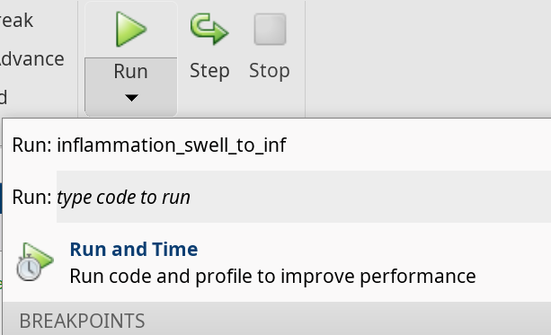
This will prompt you with a pre-filled line of code that you can modify to pass the input value.
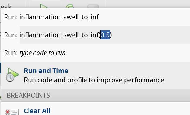
Remember to hit enter to run the code.
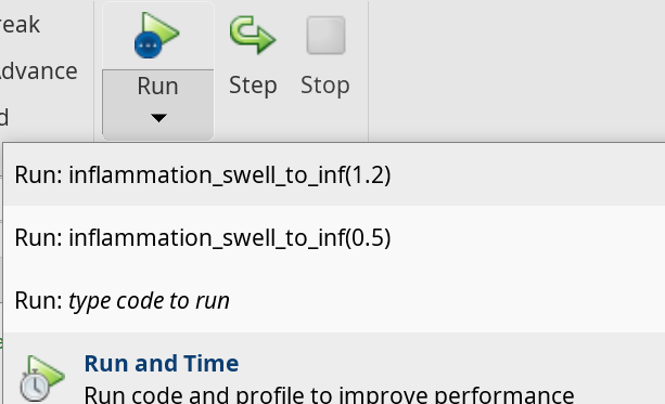
Once you’ve done that, the run code will use that value without having to go into the dropdown menu. You’ll also find the option to run the code with your specified values in the drop-down menu. You can add different input values to the code and run it again.
We got the number we expected, and at first glance it seems like it
is almost the same as a script. However, if you look at the variables in
the workspace, you’ll notice one big difference. Although a variable
called inf was defined in the function, it does not exist
in our workspace.
Lets have a look using the debugger to see what is happening.
When we pass a value, like 0.5, to the function, it is
assigned to the variable swell so that it can be used in
the body of the function. To return a value from the function, we must
assign that value to the variable inf from our function
definition line. What ever value inf has when the
end keyword in the function definition is reached, that
will be the value returned.
Outside the function, the variables swell,
inf, A, and B aren’t accessible;
they are only used by in function body.
This is one of the major differences between scripts and functions: a script automates the command line, with full access to all variables in the base workspace, whereas a function has its own separate workspace.
To be able to access variables from your workspace inside a function, you have to pass them in as inputs. To be able to save variables to your workspace from inside your function, the function needs to return them as outputs.
As with any operation, if we want to save the result, we need to assign the result to a variable, for example:
OUTPUT
val_in_inf = 1.6869And we can see val_in_inf saved in our workspace.
Writing your own conversion function
We’d like a function that reverses the conversion of Swellocity to
Inflammatons. Re-arrange the conversion formula and write a function
called inflammation_inf_to_swell that converts inflammation
measured in Inflammatons to inflammation measured in Swellocity.
Remember to save your function definition in a file with the required
name, start the file with the function definition line, followed by the
function body, ending with the end keyword.
For reference the conversion formula to take inflammation measured in Swellocity to inflammation measured in Inflammatons is:
Functions that work on arrays
One of the benefits of writing functions in MATLAB is that often they will also be able to operate on an array of numerical variables for free.
This will work when each operation in the function can be applied to an array too. In our example, we are adding a number and multiplying by another, both of which work on arrays.
This will make converting the inflammation data in our files using the function we’ve just written very quick. Give it a go!
Transforming scripts into functions
In the plot_patient_inflammation_option script we
created in the previous episode, we can choose which patient to by
modifying the variable patient_number, and whether to show
on screen or save by modifying the variable save_plots.
Because it is a script, we need to open the script, modify the
variables, save and then run it. This is a lot of steps for such a
simple request.
Can we use what we’ve learned about writing functions to transform (or refactor) our script into a function, increasing its usefulness in the process?
We already have a .m file called
plot_patient_inflammation_option, so lets begin by defining
a function with that name.
Open the plot_patient_inflammation_option.m file, if you
don’t already have it open. Instead of lines 5 and 7, where
save_plots and patient_number are set, we want
to provide the variables as inputs.
So lets remove those lines, and right at the top of our script we’ll
add the function definition, telling MATLAB what our function is called
and what inputs it needs. The function will take the variables
patient_number and save_plots as inputs, which
will decide which patient is plotted and whether the plot is saved or
displayed on screen.
MATLAB
function plot_patient_inflammation_option(patient_number, save_plots)
   % PLOT_PATIENT_INFLAMMATION_OPTION   Plots daily average, max and min inflammation.
   %    Inputs:
   %       patient_number - The patient number to plot
   %       save_plots - A boolean to decide whether to save the plot to disk (if true) or display it on screen (if false).
   %    Sample usage:
   %       plot_patient_inflammation_option(5, false)

   pn_string = num2str(patient_number);

   % Load patient data
   patient_data = readmatrix("data/base/inflammation-01.csv");
   per_day_mean = mean(patient_data);
   per_day_max = max(patient_data);
   per_day_min = min(patient_data);
   patient = patient_data(patient_number,:);
   day_of_trial = 1:40;

   if save_plots == true
      figure(visible='off')
   else
      figure
   end
   clf;

   % Define tiled layout and labels
   tlo = tiledlayout(1,2);
   xlabel(tlo,"Day of trial")
   ylabel(tlo,"Inflammation")

   % Plot average inflammation per day with the patient data
   nexttile
   title("Average")
   hold on
   plot(day_of_trial, per_day_mean, "DisplayName", "Mean")
   plot(day_of_trial, patient, "DisplayName", "Patient " + pn_string)
   legend
   hold off

   % Plot max and min inflammation per day with the patient data
   nexttile
   title("Max and Min")
   hold on
   plot(day_of_trial, per_day_max, "DisplayName", "Max")
   plot(day_of_trial, patient, "DisplayName", "Patient " + pn_string)
   plot(day_of_trial, per_day_min, "DisplayName", "Min")
   legend
   hold off

   if save_plots == true
      % Save plot in "results" folder as png image:
      saveas(fig,"results/patient_" + pn_string + ".png")

      close(fig)
end
Congratulations! You’ve now created a MATLAB function from a MATLAB script!
You may have noticed that the code inside the function is indented. MATLAB does not need this, but it makes it much more readable!
Lets clear our workspace and run our function in the command line:
You will see the plot for patient 13 saved in the
results folder, and the plot for patient 21 displayed on
screen.
So now we can get the patient plots of whichever patient we want, and we do not need to modify the script anymore.
However, you may have noticed that we have no variables in our workspace. Remember, inside the function the variables are created, but then they are deleted when the function ends. If we want to save them, we need to pass them as outputs.
Lets say, for example, that we want to save the data of the patient
in question. In our patient_analysis.m we already extract
the data and save it in patient, but we need to tell MATLAB
that we want the function to return it.
To do that we modify the function definition like this:
It is important that the variable name is the same that is used inside the function.
If we now run our function in the command line, we get:
And the variable p13 is saved in our workspace.
We could return more outputs if we want. For example, lets return the global mean as well. To do that, we need to specify all the outputs in square brackets, as an array. So we need to replace the function definition for:
MATLAB
function [per_day_mean,patient] = plot_patient_inflammation_option(patient_number, save_plots)To call our function now we need to provide space for all of the outputs, so in the command line, we run it as:
And now we have the global mean saved in the variable
mean.
Note If you had not provided space for all the
outputs, Matlab assumes you are only interested in the first one, so
ans would save the mean.
Separation of concerns
Now that we know how to write functions, we can start to make our code modular, separating the different parts of our program into small functions that can be reused.
Our plot_patient_inflammation_option function is already
quite long. You might remember that we have used the data loading and
preparation in other scripts. - Can you extract that section of the code
and put it into a separate function? - Then, refactor the
plot_patient_inflammation_option function to use this new
function.
For the data loading and preparation we will need the
patient_number as an input, and we will return the
per_day_mean, per_day_max,
per_day_min, patient, and
day_of_trial variables.
MATLAB
function [day, patient, mean, max, min] load_and_prepare_data(patient_number)
   % LOAD_AND_PREPARE_DATA   Load patient data and prepare it for plotting.
   %    Inputs:
   %       patient_number - The patient number to plot
   %    Outputs:
   %       day - The day of the trial
   %       patient - The patient data
   %       mean - The mean inflammation per day
   %       max - The max inflammation per day
   %       min - The min inflammation per day
   %    Sample usage:
   %       [day, patient, mean, max, min] = load_and_prepare_data(5)

   % Load patient data
   patient_data = readmatrix("data/base/inflammation-01.csv");
   per_day_mean = mean(patient_data);
   per_day_max = max(patient_data);
   per_day_min = min(patient_data);
   patient = patient_data(patient_number,:);
   day_of_trial = 1:40;
end
Then, we need to modify the
plot_patient_inflammation_option function to use this new
function.
MATLAB
function plot_patient_inflammation_option(patient_number, save_plots)
   % PLOT_PATIENT_INFLAMMATION_OPTION   Plots daily average, max and min inflammation.
   %    Inputs:
   %       patient_number - The patient number to plot
   %       save_plots - A boolean to decide whether to save the plot to disk (if true) or display it on screen (if false).
   %    Sample usage:
   %       plot_patient_inflammation_option(5, false)

   pn_string = num2str(patient_number);

   [day, patient, mean, max, min] = load_and_prepare_data(patient_number);

   if save_plots == true
      figure(visible='off')
   else
      figure
   end
   clf;

   % Define tiled layout and labels
   tlo = tiledlayout(1,2);
   xlabel(tlo,"Day of trial")
   ylabel(tlo,"Inflammation")

   % Plot average inflammation per day with the patient data
   nexttile
   title("Average")
   hold on
   plot(day, mean, "DisplayName", "Mean")
   plot(day, patient, "DisplayName", "Patient " + pn_string)
   legend
   hold off

   % Plot max and min inflammation per day with the patient data
   nexttile
   title("Max and Min")
   hold on
   plot(day, max, "DisplayName", "Max")
   plot(day, patient, "DisplayName", "Patient " + pn_string)
   plot(day, min, "DisplayName", "Min")
   legend
   hold off

   if save_plots == true
      % Save plot in "results" folder as png image:
      saveas(fig,"results/patient_" + pn_string + ".png")

      close(fig)
end
There are a few other things we could extract into separate
functions. For example, we can make functions that generate the
individual plots in each tile. This would make our
plot_patient_inflammation_option function even more
readable and modular, and would allow us to reuse the plotting functions
in other scripts.
- A MATLAB function must be saved in a text file with a
.mextension. The name of the file must be the same as the name of the function defined in the file. - Define functions using the
functionkeyword to start the definition, and close the definition with the keywordend. - Functions have an independent workspace. Access variables from your workspace inside a function by passing them as inputs. Access variables from the function returning them as outputs.
- The header of a function with inputs an outputs has the form:
function [output_1,output_2,...] = function_name(input_1,input_2,...)
- Break programs up into short, single-purpose functions with meaningful names.
Content from Repeating With Loops
Last updated on 2023-12-04 | Edit this page
Estimated time: 50 minutes
Overview
Questions
- How can I repeat the same operations on multiple values?
Objectives
- Explain what a for loop does.
- Correctly write for loops that repeat simple commands.
- Trace changes to a loop variable as the loops runs.
- Use a for loop to process multiple files.
Recall that we have twelve datasets in total. We’re going to need a better way to analyse them all than typing out commands for each one, because we’ll find ourselves writing a lot of duplicated code. Code that is repeated in two or more places will eventually be wrong in at least one as our project develops over time. Also, if we make changes in the way we analyse our datasets, we have to introduce that change in every copy of our code. To avoid all of this repetition, we have to teach MATLAB to repeat our commands, and to do that, we have to learn how to write loops.
We’ll start with an example. Suppose we want to print each character
in the word “lead” on a line of its own. One way is to use four
disp statements:
MATLAB
%LOOP_DEMO   Demo script to explain loops

word = 'lead';

disp(word(1))
disp(word(2))
disp(word(3))
disp(word(4))
OUTPUT
l
e
a
d
But this is a bad approach for two reasons:
It doesn’t scale: if we want to print the characters in a string that’s hundreds of letters long, we’d be better off typing them in.
It’s fragile: if we change
wordto a longer string, it only prints part of the data, and if we change it to a shorter one, it produces an error, because we’re asking for characters that don’t exist.
MATLAB
%LOOP_DEMO   Demo script to explain loops

word = 'tin';

disp(word(1))
disp(word(2))
disp(word(3))
disp(word(4))
OUTPUT
error: A(I): index out of bounds; value 4 out of bound 3There’s a better approach:
MATLAB
%LOOP_DEMO   Demo script to explain loops

word = 'lead';

for letter = 1:4
    disp(word(letter))
end
OUTPUT
l
e
a
d
This improved version uses a for loop to repeat an operation — in this case, printing to the screen — once for each element in an array.
The general form of a for loop is:
The for loop executes the commands in the loop
body for every value in the array collection. This
value is called the loop
variable, and we can call it whatever we like. In our example, we
gave it the name letter.
We have to terminate the loop body with the end keyword,
and we can have as many commands as we like in the loop body. But, we
have to remember that they will all be repeated as many times as there
are values in collection.
Our for loop has made our code more scalable, and less fragile. There’s still one little thing about it that should bother us. For our loop to deal appropriately with shorter or longer words, we have to change the first line of our loop by hand:
MATLAB
%LOOP_DEMO   Demo script to explain loops

word = 'tin';

for letter = 1:3
    disp(word(letter))
end
OUTPUT
t
i
n
Although this works, it’s not the best way to write our loop:
We might update
wordand forget to modify the loop to reflect that change.We could make a mistake while counting the number of letters in
word.
Fortunately, MATLAB provides us with a convenient function to write a better loop:
MATLAB
%LOOP_DEMO   Demo script to explain loops

word = 'aluminum';

for letter = 1:length(word)
    disp(word(letter))
end
OUTPUT
a
l
u
m
i
n
u
m
This is much more robust code, as it can deal with words of arbitrary length. Loops are not only for working with strings, they allow us to do repetitive calculations regardless of data type. Here’s another loop that calculates the sum of all even numbers between 1 and 10:
MATLAB
%LOOP_DEMO   Demo script to explain loops

total = 0;
for even_number = 2 : 2 : 10
    total = total + even_number;
end

disp('The sum of all even numbers between 1 and 10 is:')
disp(total)
It’s worth tracing the execution of this little program step by step.
The debugger
We can use the MATLAB debugger to trace the execution of a program.
The first step is to set a break point by clicking
just to the right of a line number on the - symbol. A red
circle will appear — this is the break point, and when we run the
script, MATLAB will pause execution at that line.
A green arrow appears, pointing to the next line to be run. To
continue running the program one line at a time, we use the
step button.
We can then inspect variables in the workspace or by hovering the
cursor over where they appear in the code, or get MATLAB to evaluate
expressions in the command window (notice the prompt changes to
K>>).
This process is useful to check your understanding of a program, in order to correct mistakes.
This process is illustrated below: 
Since we want to sum only even numbers, the loop index
even_number starts at 2 and increases by 2 with every
iteration. When we enter the loop, total is zero - the
value assigned to it beforehand. The first time through, the loop body
adds the value of the first even number (2) to the old value of
total (0), and updates total to refer to that
new value. On the next loop iteration, even_number is 4 and
the initial value of total is 2, so the new value assigned
to total is 6. After even_number reaches the
final value (10), total is 30; since this is the end of the
range for even_number the loop finishes and the
disp statements give us the final answer.
Note that a loop variable is just a variable that’s being used to record progress in a loop. It still exists after the loop is over, and we can re-use variables previously defined as loop variables as well:
OUTPUT
10Performing Exponentiation
MATLAB uses the caret (^) to perform exponentiation:
OUTPUT
125You can also use a loop to perform exponentiation. Remember that
b^x is just b*b*b*… x times.
Let a variable b be the base of the number and
x the exponent. Write a loop to compute b^x.
Check your result for b = 4 and x = 5.
Incrementing with Loops
Write a loop that spells the word “aluminum,” adding one letter at a time:
OUTPUT
a
al
alu
alum
alumi
alumin
aluminu
aluminumLooping in Reverse
In MATLAB, the colon operator (:) accepts a stride or
skip argument between the start and stop:
OUTPUT
1 4 7 10OUTPUT
11 8 5 2Using this, write a loop to print the letters of “aluminum” in reverse order, one letter per line.
OUTPUT
m
u
n
i
m
u
l
aAnalyzing patient data from multiple files
We now have almost everything we need to process multiple data files
using a loop and the plotting code in our
plot_daily_average function from the last lesson.
We will need to generate a list of data files to process, and then we can use a loop to repeat the analysis for each file.
We can use the dir command to return a structure
array containing the names of the files in the
data directory. Each element in this structure
array is a structure, containing information about
a single file in the form of named fields.
OUTPUT
files =
  12×1 struct array with fields:
    name
    folder
    date
    bytes
    isdir
    datenum
To access the name field of the first file, we can use the following syntax:
OUTPUT
inflammation-01.csvTo get the modification date of the third file, we can do:
OUTPUT
06-Nov-2023 14:34:15A good first step towards processing multiple files is to write a
loop which prints the name of each of our files. Let’s write this in a
script plot_all.m which we will then develop further:
MATLAB
%PLOT_ALL	Developing code to automate inflammation analysis

files = dir('data/base/inflammation-*.csv');

for i = 1:length(files)
	file_name = files(i).name;
	disp(file_name)
endOUTPUT
inflammation-01.csv
inflammation-02.csv
inflammation-03.csv
inflammation-04.csv
inflammation-05.csv
inflammation-06.csv
inflammation-07.csv
inflammation-08.csv
inflammation-09.csv
inflammation-10.csv
inflammation-11.csv
inflammation-12.csv
Another task is to generate the file names for the figures we’re
going to save. Let’s name the output file after the data file used to
generate the figure. So for the data set
inflammation-01.csv we will call the figure
inflammation-01.png. We can use the replace
command for this purpose.
The syntax for the replace command is like this:
So for example if we have the string big_shark and want
to get the string little_shark, we can execute the
following command:
OUTPUT
little_sharkRecall that we’re saving our figures to the results
directory. The best way to generate a path to a file in MATLAB is by
using the fullfile command. This generates a file path with
the correct separators for the platform you’re using (i.e. forward slash
for Linux and macOS, and backslash for Windows). This makes your code
more portable which is great for collaboration.
Putting these concepts together, we can now generate the paths for the data files, and the image files we want to save:
MATLAB
%PLOT_ALL	Developing code to automate inflammation analysis

files = dir('data/base/inflammation-*.csv');

for i = 1:length(files)
    file_name = files(i).name;

    % Generate string for image name
    img_name = replace(file_name, '.csv', '.png');

    % Generate path to data file and image file
    file_name = fullfile('data', 'base', file_name);
    img_name = fullfile('results',img_name);

    disp(file_name)
    disp(img_name)
end
OUTPUT
data/inflammation-01.csv
results/inflammation-01.png
data/inflammation-02.csv
results/inflammation-02.png
data/inflammation-03.csv
results/inflammation-03.png
data/inflammation-04.csv
results/inflammation-04.png
data/inflammation-05.csv
results/inflammation-05.png
data/inflammation-06.csv
results/inflammation-06.png
data/inflammation-07.csv
results/inflammation-07.png
data/inflammation-08.csv
results/inflammation-08.png
data/inflammation-09.csv
results/inflammation-09.png
data/inflammation-10.csv
results/inflammation-10.png
data/inflammation-11.csv
results/inflammation-11.png
data/inflammation-12.csv
results/inflammation-12.png
We’re now ready to modify plot_all.m to actually process
multiple data files:
MATLAB
%PLOT_ALL   Print statistics for all patients.
%           Save plots of statistics to disk.

files = dir('data/base/inflammation-*.csv');

% Process each file in turn
for i = 1:length(files)
    file_name = files(i).name;

    % Generate strings for image names:
    img_name  = replace(file_name, '.csv', '.png');

    % Generate path to data file and image file
    file_name = fullfile('data', 'base', file_name);
    img_name  = fullfile('results', img_name);

    plot_daily_average(file_name, img_name);

end
We run the modified script using its name in the Command Window:
The first three figures output to the results directory
are as shown below:
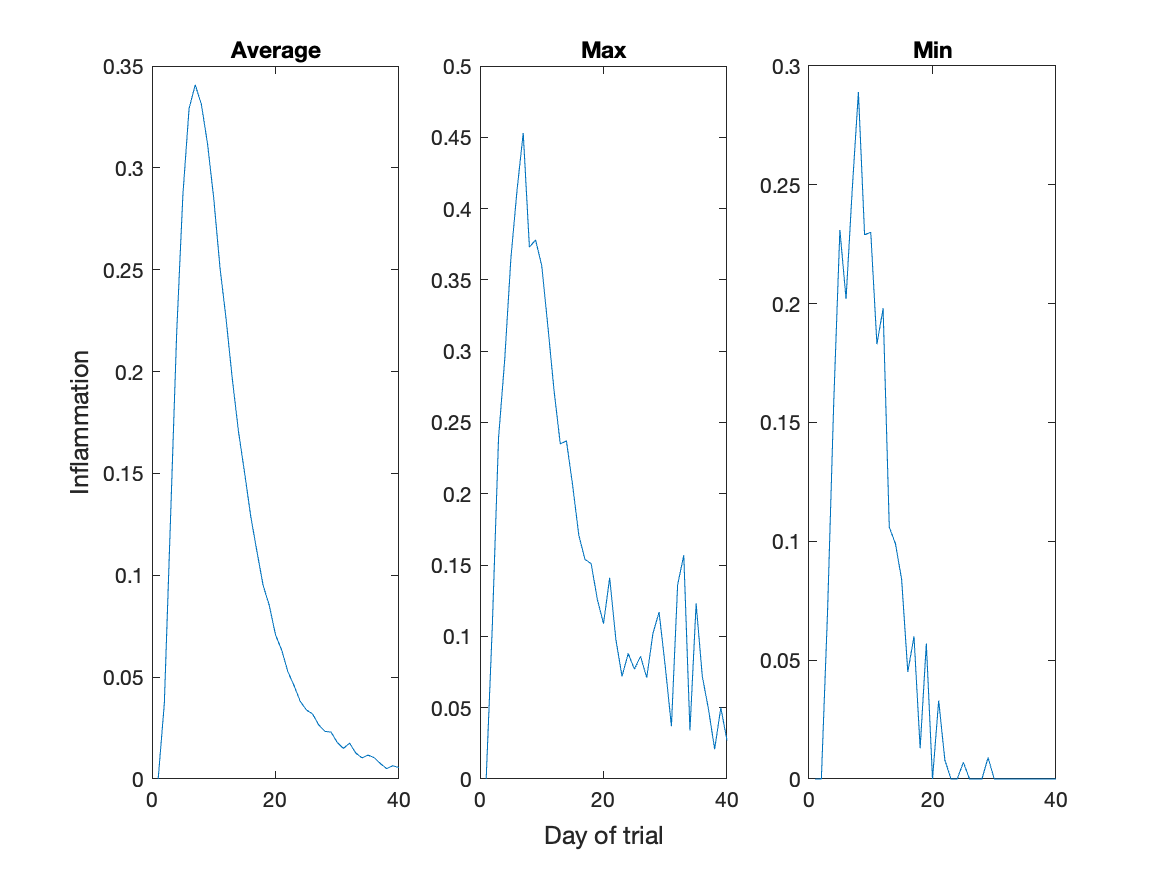
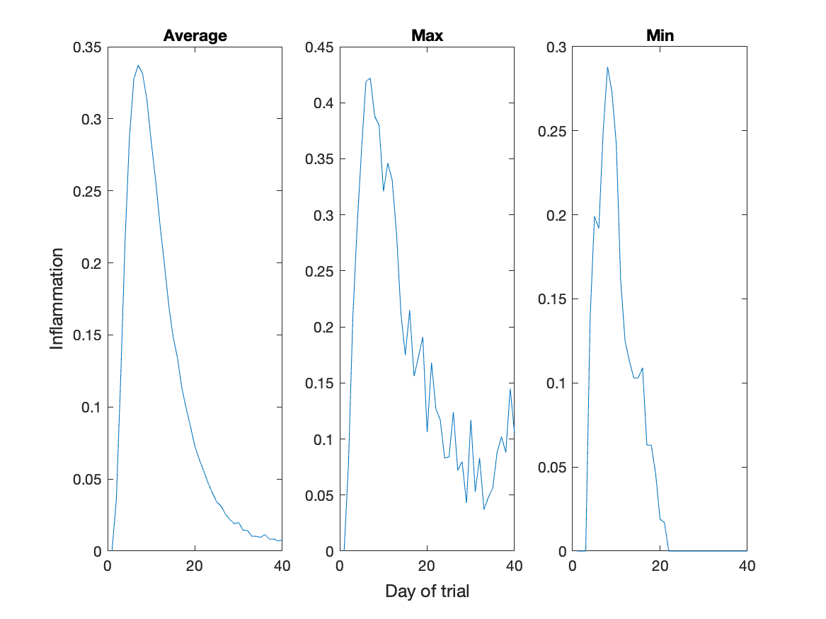
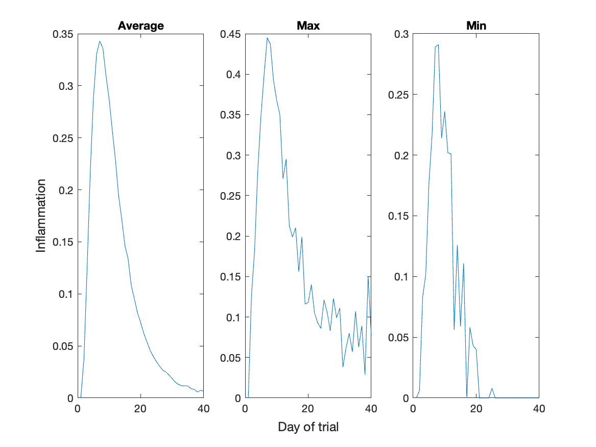
We’ve now automated the generation of these figures for all the data stored in our data folder. With minor modifications, this script could be re-used to check all our future data files.
Investigating patients with a high mean
We’re particularly interested in patients who have a mean inflammation higher than the global mean.
Write a script called plot_high_mean_patients that reads
in the file inflammation-01.csv and compares the patients
mean inflammation to the global mean. If their mean inflammation is
greater than the global inflammation, use the function
patient_vs_mean to save a plot of their inflammation to
disk for later analysis. Use both for loops and conditional statements
to do this.
Using what you’ve learned about dealing with multiple files, turn this script into a function that takes the filename of a data file as input and run it on all of the inflammation data files.
MATLAB
% PLOT_HIGH_MEAN_PATIENTS   Saves plots of patients with mean inflammation higher than the global mean inflammation.

patient_data = readmatrix('data/base/inflammation-01.csv');

per_day_mean = mean(patient_data);
global_mean =  mean(patient_data(:));

number_of_patients = size(patient_data,1);

for patient_id = 1:number_of_patients

    patient_mean = mean(patient_data(patient_id,:));

    if(patient_mean > global_mean)
        patient_reference = "Patient " + string(patient_id)
        patient_vs_mean(per_day_mean, patient_data(patient_id,:), patient_reference)
    end

end- Use
forto create a loop that repeats one or more operations.
Comments
You might have noticed that we described what we want our code to do in lines starting with the percent sign:
%. This is another plus of writing scripts: you can comment your code to make it easier to understand when you come back to it after a while.