Introduction to R and RStudio

Overview

Teaching: 60 min
Exercises: 15 min

Questions

How to find your way around RStudio?

How to interact with R?

Objectives

Describe the purpose and use of each pane in the RStudio IDE

Locate buttons and options in the RStudio IDE

Define a variable

Assign data to a variable

Manage a workspace in an interactive R session

Use mathematical and comparison operators

Call functions

Understand the concept of a vector

Understand how to extract elements from a vector

Motivation

Science is a multi-step process: once you’ve designed an experiment and collected data, the real fun begins! This lesson will teach you how to start this process using R and RStudio. We will begin with raw data, perform exploratory analyses, and learn how to plot results graphically. This example starts with a dataset from gapminder.org containing population information for many countries through time. Can you read the data into R? Can you plot the population for Senegal? Can you calculate the average income for countries on continent of Asia? By the end of these lessons you will be able to do things like plot the populations for all of these countries in under a minute!

Before Starting The Workshop

If you are using your own computer, please ensure you have the latest version of R and RStudio installed on your machine. This is important, as some packages used in the workshop may not install correctly (or at all) if R is not up to date.

Download and install the latest version of R here

Download and install RStudio here

The University machines already have suitable versions of R and RStudio installed.

Introduction to RStudio

Throughout this lesson, we’re going to teach you some of the fundamentals of the R language as well as some best practices for organizing code for scientific projects that will make your life easier.

We’ll be using RStudio: a free, open source R integrated development environment. It provides a built in editor, works on all platforms (including on servers) and provides many advantages such as integration with version control and project management.

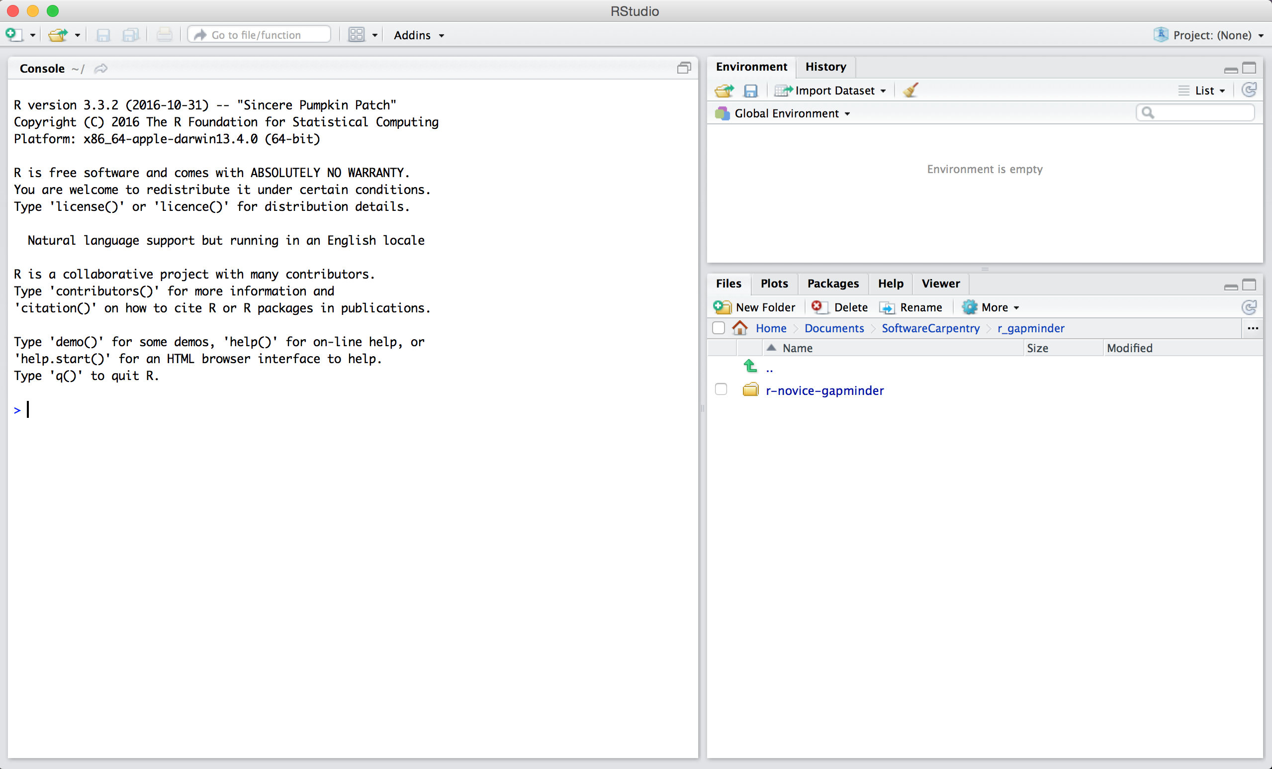
Basic layout

When you first open RStudio, you will be greeted by three panels:

The interactive R console (entire left)
Environment/History (tabbed in upper right)
Files/Plots/Packages/Help/Viewer (tabbed in lower right)

RStudio layout

Projects in R studio

When we are performing an analysis we will typically be using many files… input data, files containing code to perform the analysis, and results. By creating a project in Rstudio we make it easier to manage these files.

Let’s start the course by making a new project in RStudio, and copying the data we’ll be using for the rest of the day into it.

Click the “File” menu button, then “New Project”.
Click “New Directory”.
Click “Empty Project”.
Type in the name of the directory to store your project, e.g. “r_course”. You should avoid using spaces and full stops in the project name.
If you are using a teaching cluster machine, choose “Browse” and select P:\.
Click the “Create Project” button.

Good practices for project organization

Although there is no “best” way to lay out a project, there are some general principles to adhere to that will make project management easier:

Treat data as read only

This is probably the most important goal of setting up a project. Data is typically time consuming and/or expensive to collect. Working with them interactively (e.g., in Excel) where they can be modified means you are never sure of where the data came from, or how it has been modified since collection. It is therefore a good idea to treat your data as “read-only”.

Data Cleaning

In many cases your data will be “dirty”: it will need significant preprocessing to get into a format R (or any other programming language) will find useful. This task is sometimes called “data munging”. I find it useful to store these scripts in a separate folder, and create a second “read-only” data folder to hold the “cleaned” data sets.

Treat generated output as disposable

Anything generated by your scripts should be treated as disposable: it should all be able to be regenerated from your scripts.

There are lots of different ways to manage this output. I find it useful to have an output folder with different sub-directories for each separate analysis. This makes it easier later, as many of my analyses are exploratory and don’t end up being used in the final project, and some of the analyses get shared between projects.

Tip: Good Enough Practices for Scientific Computing

Good Enough Practices for Scientific Computing gives the following recommendations for project organization:

Put each project in its own directory, which is named after the project.

Put text documents associated with the project in the doc directory.

Put raw data and metadata in the data directory, and files generated during clean-up and analysis in a results directory.

Put source for the project’s scripts and programs in the src directory, and programs brought in from elsewhere or compiled locally in the bin directory.

Name all files to reflect their content or function.

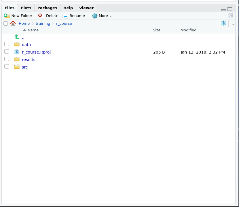
Create data, src, and results directories in your project directory.

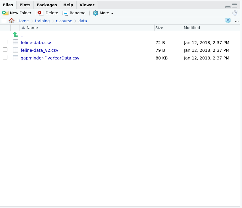
Copy the files gapminder-FiveYearData.csv, feline-data.csv, and feline-data_v2.csv files from the zip file you downloaded as part of the lesson set up to the data/ folder within your project. We will load and use these files later in the course.

Note that you cannot drag and drop files from Windows Explorer (or your operating system’s equivalent) into the files window in RStudio. You can get a new Windows Explorer (or equivalent) window for the location shown in the the files tab of RStudio by clicking “More” and selecting “Show folder in new window”. You can then drag and drop the the required files into the folder.

You may find that you need to click the “refresh” icon in RStudio’s file window before the files appear in RStudio.

Your project structure should look like this:

The data directory should looks like this:

Note that the path (“Home > training > …”) will vary according to where you created the project.

Now when we start R in this project directory, or open this project with RStudio, all of our work on this project will be entirely self-contained in this directory.

R’s working directory determines where files will be loaded from and saved to by default. The current working directory is shown above the console. If this is not our project’s directory you can set your working directory as follows:

Check that the files tab is in your project directory (or navigate there if not)
Press the More button
Select Set as current working directory

Introduction to R

Much of your time in R will be spent in the R interactive console. This console in RStudio is the same as the one you would get if you typed in R in your command-line environment.

The first thing you will see in the R interactive session is a bunch of information, followed by a > and a blinking cursor. It operates on the idea of a “Read, evaluate, print loop”: you type in commands, R tries to execute them, and then returns a result.

Using R as a calculator

The simplest thing you could do with R is do arithmetic:

1 + 100

[1] 101

And R will print out the answer, with a preceding [1]. Don’t worry about this for now, we’ll explain that later. For now think of it as indicating output.

Like bash, if you type in an incomplete command, R will wait for you to complete it:

> 1 +

Any time you hit return and the R session shows a + instead of a >, it means it’s waiting for you to complete the command. If you want to cancel a command you can press Escape and RStudio will give you back the > prompt. This can also be used to interrupt a long-running job.

When using R as a calculator, the order of operations is the same as you would have learned back in school.

From highest to lowest precedence:

Parentheses: (, )
Exponents: ^ or **
Divide: /
Multiply: *
Add: +
Subtract: -

3 + 5 * 2

[1] 13

Use parentheses to group operations in order to force the order of evaluation if it differs from the default, or to make clear what you intend.

(3 + 5) * 2

[1] 16

This can get unwieldy when not needed, but clarifies your intentions. Remember that others may later read your code.

(3 + (5 * (2 ^ 2))) # hard to read
3 + 5 * 2 ^ 2       # clear, if you remember the rules
3 + 5 * (2 ^ 2)     # if you forget some rules, this might help

The text after each line of code is called a “comment”. Anything that follows after the hash symbol # is ignored by R when it executes code.

Saving our commands

Although we can use R in this interactive way, we will usually write our commands into a file. This way we (and others) can follow the steps performed in our analysis, and we (and others) can re-run them if required.

We can create a new script by choosing the menu item: File, New File, R script, or with the keyboard shortcut Ctrl + Shift + N. Commands we type in here won’t be excuted immediately.

Script files are text files. By convention they have the extension .R.

You can execute the command that the cursor is currently on by pressing Ctrl+Enter (the cursor does not have to be at the start of the command, and the command can extend over more than one line, provided a single line does not make a complete command — you will explore this in the challenge below).

If you have selected some code, Ctrl+Enter will execute the selection.

To run all of the code in the script, press Ctrl+Shift+Enter.

Version Control

It is always a good idea to use version control with your projects.
This makes it easy to undo changes to your code, scripts and documents, and to collaborate with others. We don’t cover version control in this course, however Research IT offers a course on using git (logon required). Git is a popular version control system, that integrates well with Rstudio. Git makes collaboration with others easy when it is used in conjunction with github.

The history tab

RStudio keeps a log of the command you’ve entered. This makes it easier to go back and edit a command if you’ve made a mistake in it. There are several ways of accessing the command history:

In the console window, the up and down arrows will take you through the command history. (The command can then be edited using the left and right arrow keys)

The history tab in the top right of RStudio contains the command history. One or more lines from this can be selected. These can then be copied to the console, or to your R script by pressing the appropriate button.

Mathematical functions

R has many built in mathematical functions. To call a function, we simply type its name, followed by open and closing parentheses. Anything we type inside the parentheses are called the function’s arguments:

sin(1)  # trigonometry functions

[1] 0.841471

log(1)  # natural logarithm

[1] 0

log10(10) # base-10 logarithm

[1] 1

exp(0.5) # e^(1/2)

[1] 1.648721

Remembering function names and arguments

Don’t worry about trying to remember every function in R. You can simply look them up on Google, or if you can remember the start of the function’s name, type the start of it, then press the tab key. This will show a list of functions whose name matches what you’ve typed so far; this is known as tab completion, and can save a lot of typing (and reduce the risk of typing errors). Tab completion works in R (i.e. running it out of RStudio), and in RStudio. In RStudio this feature is even more useful; a extract of the function’s help file will be shown alongside the function name.

This is one advantage that RStudio has over R on its own: it has auto-completion abilities that allow you to more easily look up functions, their arguments, and the values that they take.

Typing a ? before the name of a command will open the help page for that command. As well as providing a detailed description of the command and how it works, scrolling to the bottom of the help page will usually show a collection of code examples which illustrate command usage. We’ll go through an example later.

Comparing things

We can also do comparison in R:

1 == 1  # equality (note two equals signs, read as "is equal to")

[1] TRUE

1 != 2  # inequality (read as "is not equal to")

[1] TRUE

1 < 2  # less than

[1] TRUE

1 <= 1  # less than or equal to

[1] TRUE

1 > 0  # greater than

[1] TRUE

1 >= -9 # greater than or equal to

[1] TRUE

Tip: Comparing Numbers

A word of warning about comparing numbers: you should never use == to compare two numbers unless they are integers (a data type which can specifically represent only whole numbers).

Computers may only represent decimal numbers with a certain degree of precision, so two numbers which look the same when printed out by R, may actually have different underlying representations and therefore be different by a small margin of error (called Machine numeric tolerance).

Instead you should use the all.equal function.

Further reading: http://floating-point-gui.de/

Variables and assignment

We can store values in variables using the assignment operator <-, like this:

x <- 1/40

Notice that assignment does not print a value. Instead, we stored it for later in something called a variable. x now contains the value 0.025:

[1] 0.025

More precisely, the stored value is a decimal approximation of this fraction called a floating point number.

Look for the Environment tab in one of the panes of RStudio, and you will see that x and its value have appeared. Our variable x can be used in place of a number in any calculation that expects a number:

log(x)

[1] -3.688879

Notice also that variables can be reassigned:

x <- 100

x used to contain the value 0.025 and and now it has the value 100.

Assignment values can contain the variable being assigned to:

x <- x + 1 #notice how RStudio updates its description of x on the top right tab

The right hand side of the assignment can be any valid R expression. The right hand side is fully evaluated before the assignment occurs.

Legal variable names

Variable names can contain letters, numbers, underscores and periods. They cannot start with a number or underscore, nor contain spaces at all. Different people use different conventions for long variable names, these include:

periods.between.words

underscores_between_words

camelCaseToSeparateWords

What you use is up to you, but be consistent.

Variables that start with a “.” are hidden variables. These will not appear in the environment window or when we use the ls() function (unless we us ls(all.names = TRUE). The ls() function is introduced in the next episode. Hidden variables are used for things such as storing R’s random number seed, which we typically don’t want to change within a session.

It is also possible to use the = operator for assignment:

x = 1/40

But this is much less common among R users. It is a good idea to be consistent with the operator you use.

We aren’t limited to storing numbers in variables:

sentence <- "the cat sat on the mat"

Note that we need to put strings of characters inside quotes.

But the type of data that is stored in a variable affects what we can do with it:

x + 1

[1] 1.025

sentence + 1

Error in sentence + 1: non-numeric argument to binary operator

We will discuss the important concept of data types in the next episode.

Challenge 1

Which of the following are valid R variable names?
min_height
max.height
_age
MaxLength
min-length
2widths
celsius2kelvin
You can use the rules described above to work out which are valid variable names, or try to assign a value to a variable and see whether R gives an error; for example:
min_height <- 2
Solution to challenge 1

The following can be used as R variables:
min_height
max.height
MaxLength
celsius2kelvin
The following will not be able to be used to create a variable
_age
min-length
2widths

Challenge 2

What will be the value of each variable after each statement in the following program?
mass <- 47.5
age <- 122
mass <- mass * 2.3
age <- age - 20
Solution to challenge 2
mass <- 47.5
This will give a value of 47.5 for the variable mass
age <- 122
This will give a value of 122 for the variable age
mass <- mass * 2.3
This will multiply the existing value of 47.5 by 2.3 to give a new value of 109.25 to the variable mass.
age <- age - 20
This will subtract 20 from the existing value of 122 to give a new value of 102 to the variable age.

Challenge 3

Run the code from the previous challenge, and write a command to compare mass to age. Is mass larger than age?
Solution to challenge 3

One way of answering this question in R is to use the > to set up the following:
mass > age
[1] TRUE
This will yield a boolean value of TRUE since 109.25 is greater than 102.

In practice, this probably isn’t an appropriate comparison to make; it doesn’t make sense to compare a mass to an age. R has no concept of units like kg and years; the values stored in the variables are just numbers. It’s our job to make sure the code we write makes appropriate comparisons.

Vectorization

As well as dealing with single values, we can work with vectors of values.
There are various ways of creating vectors; the : operator will generate sequences of consecutive values:

1:5

[1] 1 2 3 4 5

-3:3

[1] -3 -2 -1  0  1  2  3

5:1

[1] 5 4 3 2 1

The result of the : operator is a vector; this is a 1 dimensional array of values. We can apply functions to all the elements of a vector:

(1:5) * 2

[1]  2  4  6  8 10

2^(1:5)

[1]  2  4  8 16 32

We can assign a vector to a variable:

x <- 5:10

We can also create vectors “by hand” using the c() function; this tersely named function is used to combine values into a vector; these values can, themselves, be vectors:

c(2, 4, -1)

[1]  2  4 -1

c(x, 2, 2, 3)

[1]  5  6  7  8  9 10  2  2  3

Vectors aren’t limited to storing numbers:

c("a", "b", "c", "def")

[1] "a"   "b"   "c"   "def"

R comes with a few built in constants, containing useful values:

LETTERS
letters
month.abb
month.name

We will use some of these in the examples that follow.

Vector lengths

We can calculate how many elements a vector contains using the length() function:

length(x)

[1] 6

length(letters)

[1] 26

Subsetting vectors

Having defined a vector, it’s often useful to extract parts of a vector. We do this with the [] operator. Using the built in month.name vector:

month.name[2]

[1] "February"

month.name[2:4]

[1] "February" "March"    "April"

Let’s unpick the second example; 2:4 generates the sequence 2,3,4. This gets passed to the extract operator []. We can also generate this sequence using the c() function:

month.name[c(2,3,4)]

[1] "February" "March"    "April"

Vector numbering in R starts at 1

In many programming languages (C and python, for example), the first element of a vector has an index of 0. In R, the first element is 1.

Values are returned in the order that we specify the indices. We can extract the same element more than once:

month.name[4:2]

[1] "April"    "March"    "February"

month.name[c(1,1,2,3,4)]

[1] "January"  "January"  "February" "March"    "April"

Challenge 4

Return a vector containing the letters of the alphabet in reverse order
Solution to challenge 4

We can extract the elements in reverse order by generating the sequence 26, 25, … 1 using the : operator:
letters[26:1]
 [1] "z" "y" "x" "w" "v" "u" "t" "s" "r" "q" "p" "o" "n" "m" "l" "k" "j" "i" "h"
[20] "g" "f" "e" "d" "c" "b" "a"
Although this works, it makes the assumption that letters will always be length 26. Although this is probably a safe assumption in English, other languages may have more (or fewer) letters in their alphabet. It is good practice to avoid assuming anything about your data.

We can avoid assuming letters is length 26, by using the length() function:
letters[length(letters):1]
 [1] "z" "y" "x" "w" "v" "u" "t" "s" "r" "q" "p" "o" "n" "m" "l" "k" "j" "i" "h"
[20] "g" "f" "e" "d" "c" "b" "a"

If we try and extract an element that doesn’t exist in the vector, the missing values are NA:

month.name[10:13]

[1] "October"  "November" "December" NA

Missing data

NA is a special value, that is used to represent “not available”, or “missing”. If we perform computations which include NA, the result is usually NA:

1 + NA

[1] NA

This raises an interesting point; how do we test if a value is NA? This doesn’t work:

x <- NA
x == NA

[1] NA

Handling special values

There are a number of special functions you can use to handle missing data, and other special values:

is.na will return all positions in a vector, matrix, or data.frame containing NA.
likewise, is.nan, and is.infinite will do the same for NaN and Inf.
is.finite will return all positions in a vector, matrix, or data.frame that do not contain NA, NaN or Inf.
na.omit will filter out all missing values from a vector

Skipping and removing elements

If we use a negative number as the index of a vector, R will return every element except for the one specified:

month.name[-2]

 [1] "January"   "March"     "April"     "May"       "June"      "July"     
 [7] "August"    "September" "October"   "November"  "December" 

We can skip multiple elements:

month.name[c(-1, -5)]  # or month.name[-c(1,5)]

 [1] "February"  "March"     "April"     "June"      "July"      "August"   
 [7] "September" "October"   "November"  "December" 

R’s results prompt

We saw that R returns results prefixed with a [1]. This is the index of the first element of the results vector on that line of results. This is useful if we’re returning vectors that are too long to fit on a single row.

Tip: Order of operations

A common error occurs when trying to skip slices of a vector. Most people first try to negate a sequence like so:
month.name[-1:3]
This gives a somewhat cryptic error:
Error in month.name[-1:3]: only 0's may be mixed with negative subscripts
But remember the order of operations. : is really a function, so what happens is it takes its first argument as -1, and second as 3, so generates the sequence of numbers: -1, 0, 1, 2, 3.

The correct solution is to wrap that function call in brackets, so that the - operator is applied to the sequence:
-(1:3)
[1] -1 -2 -3
month.name[-(1:3)]
[1] "April"     "May"       "June"      "July"      "August"    "September"
[7] "October"   "November"  "December" 

Subsetting with logical vectors

As well as providing a list of indices we want to keep (or delete, if we prefix them with -), we can pass a logical vector to R indicating the indices we wish to select:

fourmonths <- month.name[1:4]
fourmonths

[1] "January"  "February" "March"    "April"

fourmonths[c(TRUE, FALSE, TRUE, TRUE)]

[1] "January" "March"   "April"

What happens if we supply a logical vector that is shorter than the vector we’re extracting the elements from?

fourmonths[c(TRUE,FALSE)]

[1] "January" "March"

This illustrates the idea of vector recycling; the [] extract operator “recycles” the subsetting vector:

fourmonths[c(TRUE,FALSE,TRUE,FALSE)]

[1] "January" "March"

This can be useful, but can easily catch you out.

The idea of selecting elements of a vector using a logical subsetting vector may seem a bit esoteric, and a lot more typing than just selecting the elements you want by index. It becomes really useful when we write code to generate the logical vector:

my_vector <- c(0.01, 0.69, 0.51, 0.39)
my_vector > 0.5

[1] FALSE  TRUE  TRUE FALSE

my_vector[my_vector > 0.5]

[1] 0.69 0.51

Tip: Combining logical conditions

There are many situations in which you will wish to combine multiple logical criteria. For example, we might want to find all the elements that are between two values. Several operations for combining logical vectors exist in R:

&, the “logical AND” operator: returns TRUE if both the left and right are TRUE.

|, the “logical OR” operator: returns TRUE, if either the left or right (or both) are TRUE.

The recycling rule applies with both of these, so TRUE & c(TRUE, FALSE, TRUE) will compare the first TRUE on the left of the & sign with each of the three conditions on the right.

You may sometimes see && and || instead of & and |. These operators do not use the recycling rule: they only look at the first element of each vector and ignore the remaining elements. The longer operators are mainly used in programming, rather than data analysis.

!, the “logical NOT” operator: converts TRUE to FALSE and FALSE to TRUE. It can negate a single logical condition (e.g. !TRUE becomes FALSE), or a whole vector of conditions(e.g. !c(TRUE, FALSE) becomes c(FALSE, TRUE)).

Additionally, you can compare the elements within a single vector using the all function (which returns TRUE if every element of the vector is TRUE) and the any function (which returns TRUE if one or more elements of the vector are TRUE).

Challenge 5

Given the following code:
x <- c(5.4, 6.2, 7.1, 7.5, 4.8)
x
[1] 5.4 6.2 7.1 7.5 4.8
Come up with at least 3 different commands that will produce the following output:
[1] 6.2 7.1 7.5
After you find 3 different commands, compare notes with your neighbour. Did you have different strategies?
Solution to challenge 5
x[2:4]
[1] 6.2 7.1 7.5
x[-c(1,5)]
[1] 6.2 7.1 7.5
x[c(2,3,4)]
[1] 6.2 7.1 7.5
x[c(FALSE, TRUE, TRUE, TRUE, FALSE)]
[1] 6.2 7.1 7.5
(We can use vector recycling to make the previous example slightly shorter:
x[c(FALSE, TRUE, TRUE, TRUE)]
[1] 6.2 7.1 7.5
The first element of the logical vector will be recycled)

We can construct a logical test to generate the logical vector:
x[x > 6]
[1] 6.2 7.1 7.5
Unpicking this example, x > 6 generates the logical vector:
[1] FALSE  TRUE  TRUE  TRUE FALSE
Which is passed to the [ ] subsetting operator.

Data types

One thing you may have noticed is that all the data in a vector has been the same type; all the elements have had the same type (i.e. they have all been numbers, all been character, or all been logical (TRUE/FALSE)). This is an important property of vectors; the type of data the vector holds is a property of the vector, not of each element. Let’s look at what happens if we try to create a vector of numeric and character data:

c(1, 2, "three", "four", 5)

[1] "1"     "2"     "three" "four"  "5"

We see that R has coerced the elements containing digits to strings, so that all the elements have the same type. We will talk more about data types in a later episode.

Managing your environment (self study)

In this section we will discuss ways of keeping your environment tidy.

ls will list all of the variables and functions stored in the global environment (your working R session):

ls()

[1] "x"

Information on the objects in your environment is also available from the environment panel in RStudio.

Tip: hidden objects

Like in the shell, ls will hide any variables or functions starting with a . by default. To list all objects, type ls(all.names=TRUE) instead

Note here that we didn’t given any arguments to ls, but we still needed to give the parentheses to tell R to call the function.

You can use rm to delete objects you no longer need. To delete x:

x <- 5
x

[1] 5

rm(x)
# x has now been deleted; so trying to access it will give an error
x

Error in eval(expr, envir, enclos): object 'x' not found

If you have lots of things in your environment and want to delete all of them, you can pass the results of ls to the rm function:

rm(list = ls())

In this case we’ve combined the two. Like the order of operations, anything inside the innermost parentheses is evaluated first, and so on.

In this case we’ve specified that the results of ls should be used for the list argument in rm. When assigning values to arguments by name, you must use the = operator, and not <-.

If instead we use <-, there will be unintended side effects, or you may get an error message:

rm(list <- ls())

Error in rm(list <- ls()): ... must contain names or character strings

Tip: Warnings vs. Errors

Pay attention when R does something unexpected! Errors, like above, are thrown when R cannot proceed with a calculation. Warnings on the other hand usually mean that the function has run, but it probably hasn’t worked as expected.

In both cases, the message that R prints out usually give you clues how to fix a problem.

Comments

If we include the # symbol in a command in R, everything following it will be ignored. This lets us enter comments into our code.

Key Points

Use RStudio to write and run R programs.

R has the usual arithmetic operators and mathematical functions.

Use <- to assign values to variables.

Use the [] operator to extract elements from a vector

lesson home

Data analysis using R

next episode

Introduction to R and RStudio

Overview

Motivation

Before Starting The Workshop

Introduction to RStudio

Projects in R studio

Good practices for project organization

Treat data as read only

Data Cleaning

Treat generated output as disposable

Tip: Good Enough Practices for Scientific Computing

Introduction to R

Using R as a calculator

Saving our commands

Version Control

The history tab

Mathematical functions

Remembering function names and arguments

Comparing things

Tip: Comparing Numbers

Variables and assignment

Legal variable names

Challenge 1

Solution to challenge 1

Challenge 2

Solution to challenge 2

Challenge 3

Solution to challenge 3

Vectorization

Vector lengths

Subsetting vectors

Vector numbering in R starts at 1

Challenge 4

Solution to challenge 4

Missing data

Handling special values

Skipping and removing elements

R’s results prompt

Tip: Order of operations

Subsetting with logical vectors

Tip: Combining logical conditions

Challenge 5

Solution to challenge 5

Data types

Managing your environment (self study)

Tip: hidden objects

Tip: Warnings vs. Errors

Comments

Key Points

lesson home

next episode