Combining your code with text

Overview

Teaching: 20 min
Exercises: 10 min

Questions

• How can I organise my work using Rmarkdown documents?

Objectives

• To understand the RMarkdown syntax

• To understand how to create and use a markdown document

• To understand how to use Knitr to write reports

Introduction

So far today we’ve written scripts to load, analyse and plot data. We’ve also discussed how to save data and plots. It can often be useful to combine our analysis and a written explanation of what we’ve done. This is different from commenting our code (which we should be doing anyway); instead we’re talking about writing up our analysis while doing it.

Jupyter / Python notebooks

This is a similar idea to a Jupyter notebook, but is integrated within R Studio.

Let’s get started by making a new notebook. From the File menu, choose New file and then Rnotebook. A new window will open containing an example notebook:

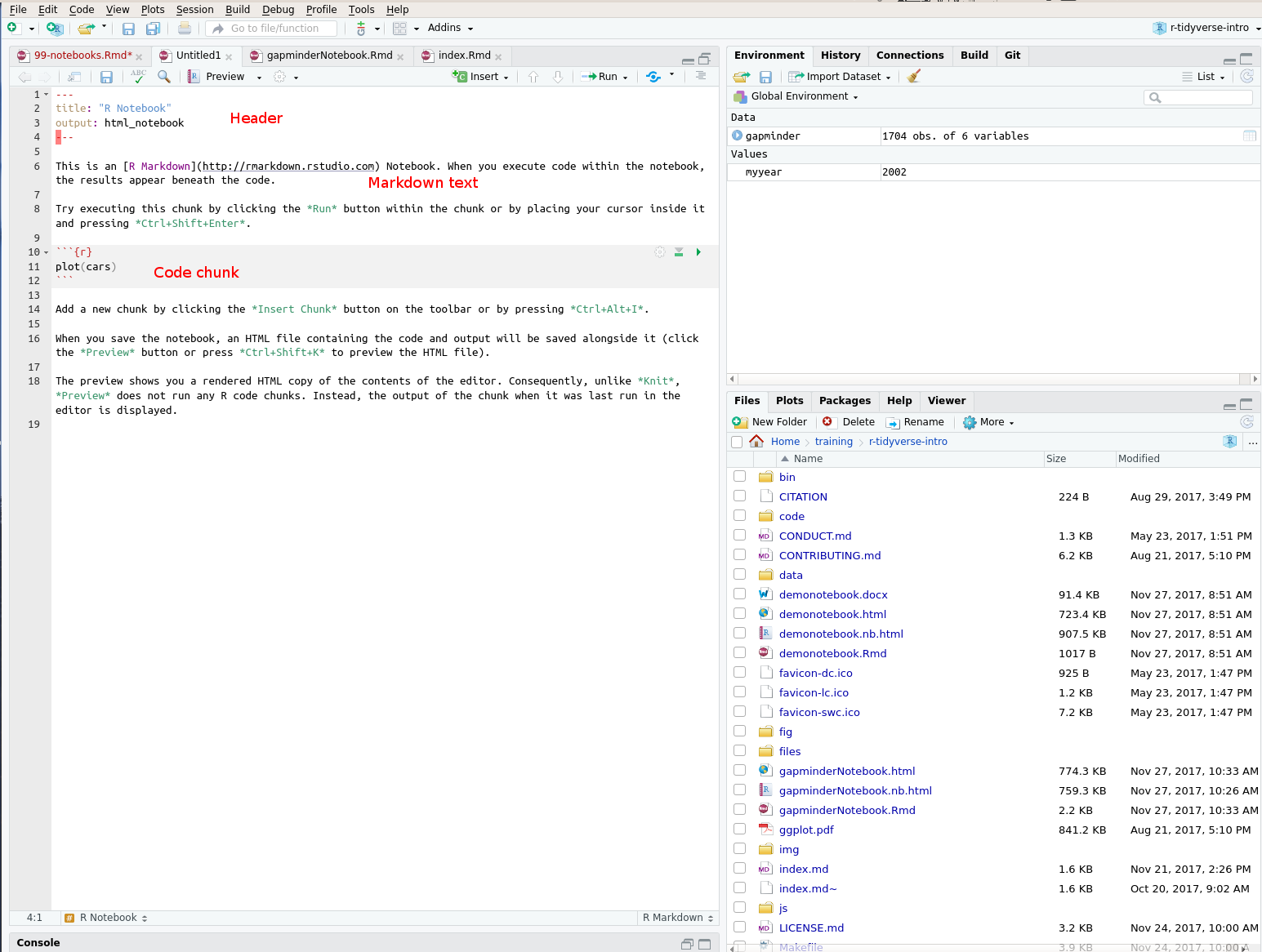
The notebook includes “chunks” of text, and chunks of R code.

The start of an R code region is marked with ` ` ` { r } The end of an code region is marked with ` ` ` These are a little awkward to type; pressing Ctrl+Alt+I will insert a new chunk of R code into your document. You can (and should) label your chunks of R code:

` ` ` { r mychunk }

This makes it easier to jump between chunks within your document, using the selector box a the lower left of the edit window.

The header at the start of the notebook (between the ---s) contains metadata which tells R how to process the notebook. This can be edited by hand (for example to change the “title:” field), or to add an “author: “ field. R Studio may also modify it, for example, if you change the output format of the document.

Before we go any further, make a new subdirectory for your notebooks, for example, notebook. and save the notebook in it using File, Save. We need to do this so that we can preview and build the notebook. When you run code in your notebook, RStudio will set the working directory to be the notebook’s directory. This means that if we want to load some data from our data folder, we will need to use the path ../data/gapminder-FiveYearData.csv (rather than data/gapminder-FiveYearData.csv, as we used previously). The .. tells R to look in the parent directory of the working directory.

We can run the notebook interactively within R Studio. Press the “Run” button (at the top of the editor window) and choose “Run all” (or press Ctrl+Shift+R). This will execute each chunk of code within R Studio and show us the results of each chunk within the document. This makes it easier to interactively edit our code, look at the results of our analysis, and edit our text within the same environment.

We can preview the notebook by selecting “Preview notebook” from the top of the editor window. This will render the text and code into an HTML document. Note that the preview will use executed chunks of R code in the editor window. For this reason it is a good idea to choose “Restart R and run all chunks” from the run button (at the top of the editor). This will ensure your code has been run in order, and that it is self consistent.

As an example of using notebooks, let’s use the gapminder data, and some of the ideas introduced earlier to run, and to document, an analysis of the data.

Challenge 1

Modify the example notebook to load the gapminder data into your working environment, and to print an extract of it in the notebook (using print(gapminder) will do this).

It is a good idea to make a separate chunk called “setup” to load your libraries and clear your working environment. You can re-use the code you used to load the gapminder data earlier today.

Solution

Because these lessons are built from R Markdown documents, it is difficult to show the markdown itself within them. The solution to this challenge can be found here

At the moment all the code and data we’ve written are shown in the document. This can be excessive. For example, we may get diagnostic messages which we don’t anticipate being of interest to the reader. We can hide the R code in a chunk as follows:

` ` ` { r mychunk echo=FALSE }

We can hide messages printed to the screen with:

` ` ` { r mychunk message=FALSE }

Note that we can exclude all of the output of a chunk with:

` ` ` { r mychunk include=FALSE }

You may need to do this to suppress package start-up messages; these are handled by R in a slightly different way from regular messages.

Options can be combined by separating them with commas:

` ` ` { r mychunk echo=FALSE, messages=FALSE }

Other options

Warnings and errors can be suppressed with “warning=FALSE” and “error=FALSE”. You should use these options with care; warnings and errors usually happen for a reason!. “eval=FALSE” will include the chunk (i.e. you’ll see the R code, provided “echo=TRUE”), but it won’t evaluate it. This can be useful when you want to avoid running a slow piece of your analysis, for example.

You can set the default options for all subsequent chunks by including, e.g., in an R code chunk:

knitr::opts_chunk$set(echo = FALSE, warning = TRUE)

You would typically include this in your setup chunk, and use include=FALSE so as not to output the code or output of the setup chunk itself.

Challenge 2

Hide the output and any messages when you load your data and libraries. Hide the command needed to preview the gapminder data.

Solution

The solution can be found here.

How much of the “behind the scenes” work you show in a notebook is up to you, and will depend on the intended audience. If you hide all the code, you can produce something which looks very much like a regular scientific paper. The benefit of writing a paper like this is that your analysis and write up are in the same place. If your analysis (or data) change, the paper will be updated automatically. By keeping the underlying R Markdown file it is possible for you, or others to work out exactly how each figure in you work was produced.

We can also display R output “inline” (i.e. so it appears as normal text within a paragraph): For example:

The sine of 0 is `r sin(0)`

Will display as:

The sine of 0 is 0

Formatting our text

We can format our notebook using markdown. For example, to make some text italic, we use:

_This text is italic._ This text isn't

Which will appear as:

This text is italic. This text isn’t

R Studio has a quick reference guide to common markdown formatting codes. This can be found under “Help”, “Markdown quick reference”. There is also a more comprehensive cheat sheet under the help menu, and an even more comprehensive reference guide.

LaTeX equations can be included in your notebook as follows:

$$a=\pi r^2$$

Which will appear as:

You can insert an equation within a line of text by enclosing the LaTeX code within single dollars.

More complicated formatting

It is also possible to combine R code and LaTeX text. This approach is better suited to producing a “static” document, such as a paper, rather than a notebook. To do this, choose “File”, “New”, “R Sweave”. R Studio will produce a skeleton document. As with notebooks, Ctrl+Shift+I will insert a new R code chunk. To display inline R code use:

The cos of 0 is \Sexpr{cos(0)}

which will display as “The cos of 0 is 1”.

Don’t repeat yourself

Writing up our work in notebooks is a really useful way of explaining our analyses to others, and our future selves. It also makes it really easy to experiment with your analysis, and to try things out. This makes it particularly important to define your parameters once, and then refer to the variable they’re stored in, rather than using them more than once.

There are two ways of doing this; we can define our parameters in a code chunk, and refer to the variables, or define a parameter in the header of the document.

Take a look at the DRYNotebook.Rmd. In this, we define the year we’re interested in as a parameter, and always refer to the parameter rather than hard-coding a year into various places in the text and code.

Challenge 3

Part 1: Modify your notebook, or use the DRYNotebook.Rmd as a starting point, to plot a line graph showing life expectancy over time, coloured by continent (you should have code to do this from the ggplot lesson).

Part 2: Modify the notebook to print something similar to the following paragraph:

“In 2002, citizens of Japan had the longest average life expectancy in the world, at 82. By comparison, in United Kingdom, the average life expectancy was 78.471”.

You should pass the year we wish to calculate the life expectancies at (e.g. 2002), and the comparator country (e.g. United Kingdom) as parameters to your report.

Hints: To calculate the country with the longest life expectancy use arrange(desc()) to sort the data in descending order. The country with the longest life expectancy will then be first in the resulting tibble.

If you save the tibble containing the data sorted by age, you can then extract a column from it, as a vector using the $ operator:

gapminderSorted$lifeExp

You can then use the indexing operator [] to get the value of the first element of this vector, which will be the largest age.

Solution

The solution can be found here

Doing more with Markdown and notebooks

We sometimes want to include the output of of statistical analysis (such as the results of the models we fitted using lm(). The pander package will add the appropriate markdown formatting to many R functions to make them display nicely. Having installed and loaded the pander package, run the pander() function on the object you wish to display, e.g.

library(pander)
pander(uk_lifeExp_model_squared)

Make sure you use the option results='asis' on the code chunk; this will allow the markdown formatting generated by pander to be processed.

In this episode we’ve looked at how to make notebooks, and how to compile these into Word, PDF and HTML files. The British Ecological Society has published an excellent guide on producing reproducible reports using RMarkdown, and on reproducible research more generally (although aimed at Ecologists the approaches they advocate are general).

The book Reproducible Research with R and RStudio, by Christopher Gandrud also explains this approach.

We can use a similar approach to produce other types of outputs. The RMarkdown gallery contains examples of the many different types of document you can produce (some of these may require a newer version of R Studio than the one installed on the PC clusters).

This course was written in R Studio. The slides I used to introduce the course at the start were written as an R Markdown document and each episode of this course is written as an R Markdown document (although the conversion to an HTML page is a little more complex than for the examples we looked at - this is so that the formatting of the challenges etc. works properly). You can see all of the underlying R Markdown for this course on Github, in the _episodes_rmd directory; having selected an episode you will need to click the “raw” button to see the markdown itself.

Key Points

• Notebooks let us combine R code and text explaining our analysis